Confidence interval

Interval estimation can be contrasted with point estimation. A point estimate is a single value given as the estimate of a population parameter that is of interest, for example, the mean of some quantity. An interval estimate specifies instead a range within which the parameter is estimated to lie. Confidence intervals are commonly reported in tables or graphs along with point estimates of the same parameters, to show the reliability of the estimates.

For example, a confidence interval can be used to describe how reliable survey results are. In a poll of election–voting intentions, the result might be that 40% of respondents intend to vote for a certain party. A 99% confidence interval for the proportion in the whole population having the same intention on the survey might be 30% to 50%. From the same data one may calculate a 90% confidence interval, which in this case might be 37% to 43%. A major factor determining the length of a confidence interval is the size of the sample used in the estimation procedure, for example, the number of people taking part in a survey.

Various interpretations of a confidence interval can be given (taking the 90% confidence interval as an example in the following).

• The confidence interval can be expressed in terms of samples (or repeated samples): "Were this procedure to be repeated on numerous samples, the fraction of calculated confidence intervals (which would differ for each sample) that encompass the true population parameter would tend toward 90%."[2]
• The confidence interval can be expressed in terms of a single sample: "There is a 90% probability that the calculated confidence interval from some future experiment encompasses the true value of the population parameter." Note this is a probability statement about the confidence interval, not the population parameter. This considers the probability associated with a confidence interval from a pre-experiment point of view, in the same context in which arguments for the random allocation of treatments to study items are made. Here the experimenter sets out the way in which they intend to calculate a confidence interval and to know, before they do the actual experiment, that the interval they will end up calculating has a particular chance of covering the true but unknown value.[4] This is very similar to the "repeated sample" interpretation above, except that it avoids relying on considering hypothetical repeats of a sampling procedure that may not be repeatable in any meaningful sense. See Neyman construction.
• The explanation of a confidence interval can amount to something like: "The confidence interval represents values for the population parameter for which the difference between the parameter and the observed estimate is not statistically significant at the 10% level".[7] In fact, this relates to one particular way in which a confidence interval may be constructed.

In each of the above, the following applies: If the true value of the parameter lies outside the 90% confidence interval, then a sampling event has occurred (namely, obtaining a point estimate of the parameter at least this far from the true parameter value) which had a probability of 10% (or less) of happening by chance.

Confidence intervals and levels are frequently misunderstood, and published studies have shown that even professional scientists often misinterpret them.[8][9][10][11][12]

• A 95% confidence level does not mean that for a given realized interval there is a 95% probability that the population parameter lies within the interval (i.e., a 95% probability that the interval covers the population parameter).[13] According to the strict frequentist interpretation, once an interval is calculated, this interval either covers the parameter value or it does not; it is no longer a matter of probability. The 95% probability relates to the reliability of the estimation procedure, not to a specific calculated interval.[14] Neyman himself (the original proponent of confidence intervals) made this point in his original paper:[4]

  "It will be noticed that in the above description, the probability statements refer to the problems of estimation with which the statistician will be concerned in the future. In fact, I have repeatedly stated that the frequency of correct results will tend to α. Consider now the case when a sample is already drawn, and the calculations have given [particular limits]. Can we say that in this particular case the probability of the true value [falling between these limits] is equal to α? The answer is obviously in the negative. The parameter is an unknown constant, and no probability statement concerning its value may be made..."

Deborah Mayo expands on this further as follows:[15]

"It must be stressed, however, that having seen the value [of the data], Neyman–Pearson theory never permits one to conclude that the specific confidence interval formed covers the true value of 0 with either (1 − α)100% probability or (1 − α)100% degree of confidence. Seidenfeld's remark seems rooted in a (not uncommon) desire for Neyman–Pearson confidence intervals to provide something which they cannot legitimately provide; namely, a measure of the degree of probability, belief, or support that an unknown parameter value lies in a specific interval. Following Savage (1962), the probability that a parameter lies in a specific interval may be referred to as a measure of final precision. While a measure of final precision may seem desirable, and while confidence levels are often (wrongly) interpreted as providing such a measure, no such interpretation is warranted. Admittedly, such a misinterpretation is encouraged by the word 'confidence'."

• A 95% confidence level does not mean that 95% of the sample data lie within the confidence interval.
• A confidence interval is not a definitive range of plausible values for the sample parameter, though it may be understood as an estimate of plausible values for the population parameter.
• A particular confidence level of 95% calculated from an experiment does not mean that there is a 95% probability of a sample parameter from a repeat of the experiment falling within this interval.[12]

Confidence intervals were introduced to statistics by Jerzy Neyman in a paper published in 1937.[16] However, it took quite a while for confidence intervals to be accurately and routinely used. In the earliest modern controlled clinical trial of a medical treatment for acute stroke, published by Dyken and White in 1959, the investigators concluded that cortisol increased the risk of stroke. When confidence interval was applied however, it showed that the no possible advantage to using cortisol statement was not strictly true. There was a 12% chance that cortisol reduced risk. Especially in the medical sciences, where datasets can be small, proper selection of confidence intervals is necessary to determine size of effect, direction, and reliably determine whether the null hypothesis can be accepted or rejected.[17]

It wasn't until the 1980s that journals required confidence intervals and p-values to be reported in papers. By 1992, imprecise estimates were still common, even for large trials. This prevented a clear decision regarding the null hypothesis. For example, a study of medical therapies for acute stroke came to the conclusion that the stroke treatments could reduce mortality or increase it by 10%–20%. Strict admittance to the study introduced unforeseen error, further increasing uncertainty in the conclusion. Studies persisted, and it wasn't until 1997 that a trial with a massive sample pool and acceptable confidence interval was able to provide a definitive answer: cortisol therapy does not reduce the risk of acute stroke.[17]

The principle behind confidence intervals was formulated to provide an answer to the question raised in statistical inference of how to deal with the uncertainty inherent in results derived from data that are themselves only a randomly selected subset of a population. There are other answers, notably that provided by Bayesian inference in the form of credible intervals. Confidence intervals correspond to a chosen rule for determining the confidence bounds, where this rule is essentially determined before any data are obtained, or before an experiment is done. The rule is defined such that over all possible datasets that might be obtained, there is a high probability ("high" is specifically quantified) that the interval determined by the rule will include the true value of the quantity under consideration. The Bayesian approach appears to offer intervals that can, subject to acceptance of an interpretation of "probability" as Bayesian probability, be interpreted as meaning that the specific interval calculated from a given dataset has a particular probability of including the true value, conditional on the data and other information available. The confidence interval approach does not allow this since in this formulation and at this same stage, both the bounds of the interval and the true values are fixed values, and there is no randomness involved. On the other hand, the Bayesian approach is only as valid as the prior probability used in the computation, whereas the confidence interval does not depend on assumptions about the prior probability.

The questions concerning how an interval expressing uncertainty in an estimate might be formulated, and of how such intervals might be interpreted, are not strictly mathematical problems and are philosophically problematic.[18] Mathematics can take over once the basic principles of an approach to 'inference' have been established, but it has only a limited role in saying why one approach should be preferred to another: For example, a confidence level of 95% is often used in the biological sciences, but this is a matter of convention or arbitration. In the physical sciences, a much higher level may be used.[19]

Confidence intervals are closely related to statistical significance testing. For example, if for some estimated parameter θ one wants to test the null hypothesis that θ = 0 against the alternative that θ ≠ 0, then this test can be performed by determining whether the confidence interval for θ contains 0.

More generally, given the availability of a hypothesis testing procedure that can test the null hypothesis θ = θ₀ against the alternative that θ ≠ θ₀ for any value of θ₀, then a confidence interval with confidence level γ = 1 − α can be defined as containing any number θ₀ for which the corresponding null hypothesis is not rejected at significance level α.[20]

If the estimates of two parameters (for example, the mean values of a variable in two independent groups) have confidence intervals that do not overlap, then the difference between the two values is more significant than that indicated by the individual values of α.[21] So, this "test" is too conservative and can lead to a result that is more significant than the individual values of α would indicate. If two confidence intervals overlap, the two means still may be significantly different.[22][23][24] Accordingly, and consistent with the Mantel-Haenszel Chi-squared test, is a proposed fix whereby one reduces the error bounds for the two means by multiplying them by the square root of ½ (0.707107) before making the comparison.[25]

While the formulations of the notions of confidence intervals and of statistical hypothesis testing are distinct, they are in some senses related and to some extent complementary. While not all confidence intervals are constructed in this way, one general purpose approach to constructing confidence intervals is to define a 100(1 − α)% confidence interval to consist of all those values θ₀ for which a test of the hypothesis θ = θ₀ is not rejected at a significance level of 100α%. Such an approach may not always be available since it presupposes the practical availability of an appropriate significance test. Naturally, any assumptions required for the significance test would carry over to the confidence intervals.

It may be convenient to make the general correspondence that parameter values within a confidence interval are equivalent to those values that would not be rejected by a hypothesis test, but this would be dangerous. In many instances the confidence intervals that are quoted are only approximately valid, perhaps derived from "plus or minus twice the standard error," and the implications of this for the supposedly corresponding hypothesis tests are usually unknown.

It is worth noting that the confidence interval for a parameter is not the same as the acceptance region of a test for this parameter, as is sometimes thought. The confidence interval is part of the parameter space, whereas the acceptance region is part of the sample space. For the same reason, the confidence level is not the same as the complementary probability of the level of significance.

Confidence regions generalize the confidence interval concept to deal with multiple quantities. Such regions can indicate not only the extent of likely sampling errors but can also reveal whether (for example) it is the case that if the estimate for one quantity is unreliable, then the other is also likely to be unreliable.

A confidence band is used in statistical analysis to represent the uncertainty in an estimate of a curve or function based on limited or noisy data. Similarly, a prediction band is used to represent the uncertainty about the value of a new data point on the curve, but subject to noise. Confidence and prediction bands are often used as part of the graphical presentation of results of a regression analysis.

Confidence bands are closely related to confidence intervals, which represent the uncertainty in an estimate of a single numerical value. "As confidence intervals, by construction, only refer to a single point, they are narrower (at this point) than a confidence band which is supposed to hold simultaneously at many points."[26]

Confidence intervals can be calculated using two different values: t-values or z-values, as shown in the basic example above. Both values are tabulated in tables, based on degrees of freedom and the tail of a probability distribution. More often, z-values are used. These are the critical values of the normal distribution with right tail probability. However, t-values are used when the sample size is below 30 and the standard deviation is unknown.[1][29]

When the variance is unknown, we must use a different estimator: ${\displaystyle S_{n}}$. This allows the formation of a distribution that only depends on ${\displaystyle n}$ and whose density can be expression explicitly.[1]

Definition: A continuous random variable has a t-distribution with parameter m, where ${\displaystyle m\geq 1}$ is an integer, if its probability density is given by ${\displaystyle f(x)=\left(k_{m}\left(1+{\frac {x^{2}}{m}}\right)\right)^{\frac {-m+1}{2}}}$ for ${\displaystyle -\infty <x<\infty }$, where ${\displaystyle k_{m}={\frac {\Gamma \left({\frac {m+1}{2}}\right)}{{\sqrt {m\pi }}\,\Gamma \left({\frac {m}{2}}\right)}}}$. This distribution is denoted by ${\displaystyle t(m)}$ and is referred to as the t-distribution with m degrees of freedom.[1]

Example: Using t-distribution table[30]

1.Find degrees of freedom (df) from sample size:

If sample size = 10, df = 9.

2. Subtract the confidence interval (CL) from 1 and then, divide it by two. This value is the alpha level. (alpha + CL = 1)

2. Look df and alpha in the t-distribution table. For df = 9 and alpha = 0.01, the table gives a value of 2.821. This value obtained from the table is the t-score.

Let X be a random sample from a probability distribution with statistical parameters θ, which is a quantity to be estimated, and φ, representing quantities that are not of immediate interest. A confidence interval for the parameter θ, with confidence level or confidence coefficient γ, is an interval with random endpoints (u(X), v(X)), determined by the pair of random variables u(X) and v(X), with the property:

${\displaystyle {\Pr }_{\theta ,\varphi }(u(X)<\theta <v(X))=\gamma {\text{ for all }}(\theta ,\varphi ).}$

The quantities φ in which there is no immediate interest are called nuisance parameters, as statistical theory still needs to find some way to deal with them. The number γ, with typical values close to but not greater than 1, is sometimes given in the form 1 − α (or as a percentage 100%·(1 − α)), where α is a small non-negative number, close to 0.

Here Pr_θ,φ indicates the probability distribution of X characterised by (θ, φ). An important part of this specification is that the random interval (u(X), v(X)) covers the unknown value θ with a high probability no matter what the true value of θ actually is.

Note that here Pr_θ,φ need not refer to an explicitly given parameterized family of distributions, although it often does. Just as the random variable X notionally corresponds to other possible realizations of x from the same population or from the same version of reality, the parameters (θ, φ) indicate that we need to consider other versions of reality in which the distribution of X might have different characteristics.

In a specific situation, when x is the outcome of the sample X, the interval (u(x), v(x)) is also referred to as a confidence interval for θ. Note that it is no longer possible to say that the (observed) interval (u(x), v(x)) has probability γ to contain the parameter θ. This observed interval is just one realization of all possible intervals for which the probability statement holds.

In many applications, confidence intervals that have exactly the required confidence level are hard to construct. But practically useful intervals can still be found: the rule for constructing the interval may be accepted as providing a confidence interval at level γ if

${\displaystyle {\Pr }_{\theta ,\varphi }(u(X)<\theta <v(X))\approx \gamma {\text{ for all }}(\theta ,\varphi )\,}$

to an acceptable level of approximation. Alternatively, some authors[31] simply require that

${\displaystyle {\Pr }_{\theta ,\varphi }(u(X)<\theta <v(X))\geq \gamma {\text{ for all }}(\theta ,\varphi )\,}$

which is useful if the probabilities are only partially identified or imprecise, and also when dealing with discrete distributions. Confidence limits of form ${\displaystyle {\Pr }_{\theta ,\varphi }(u(X)<\theta )\geq \gamma }$ and ${\displaystyle {\Pr }_{\theta ,\varphi }(\theta <v(X))\geq \gamma }$ are called conservative[32]; accordingly, one speaks of conservative confidence intervals and, in general, regions.

When applying standard statistical procedures, there will often be standard ways of constructing confidence intervals. These will have been devised so as to meet certain desirable properties, which will hold given that the assumptions on which the procedure rely are true. These desirable properties may be described as: validity, optimality, and invariance. Of these "validity" is most important, followed closely by "optimality". "Invariance" may be considered as a property of the method of derivation of a confidence interval rather than of the rule for constructing the interval. In non-standard applications, the same desirable properties would be sought.

• Validity. This means that the nominal coverage probability (confidence level) of the confidence interval should hold, either exactly or to a good approximation.
• Optimality. This means that the rule for constructing the confidence interval should make as much use of the information in the data-set as possible. Recall that one could throw away half of a dataset and still be able to derive a valid confidence interval. One way of assessing optimality is by the length of the interval so that a rule for constructing a confidence interval is judged better than another if it leads to intervals whose lengths are typically shorter.
• Invariance. In many applications, the quantity being estimated might not be tightly defined as such. For example, a survey might result in an estimate of the median income in a population, but it might equally be considered as providing an estimate of the logarithm of the median income, given that this is a common scale for presenting graphical results. It would be desirable that the method used for constructing a confidence interval for the median income would give equivalent results when applied to constructing a confidence interval for the logarithm of the median income: specifically the values at the ends of the latter interval would be the logarithms of the values at the ends of former interval.

For non-standard applications, there are several routes that might be taken to derive a rule for the construction of confidence intervals. Established rules for standard procedures might be justified or explained via several of these routes. Typically a rule for constructing confidence intervals is closely tied to a particular way of finding a point estimate of the quantity being considered.

Summary statistics

This is closely related to the method of moments for estimation. A simple example arises where the quantity to be estimated is the mean, in which case a natural estimate is the sample mean. The usual arguments indicate that the sample variance can be used to estimate the variance of the sample mean. A confidence interval for the true mean can be constructed centered on the sample mean with a width which is a multiple of the square root of the sample variance.

Likelihood theory

Where estimates are constructed using the maximum likelihood principle, the theory for this provides two ways of constructing confidence intervals or confidence regions for the estimates. One way is by using Wilks's theorem to find all the possible values of ${\displaystyle \theta }$ that fulfill the following restriction:[33]

${\displaystyle \ln(L(\theta ))\geq \ln(L({\hat {\theta }}))-{\frac {1}{2}}\chi _{1,1-\alpha }^{2}}$

Estimating equations

The estimation approach here can be considered as both a generalization of the method of moments and a generalization of the maximum likelihood approach. There are corresponding generalizations of the results of maximum likelihood theory that allow confidence intervals to be constructed based on estimates derived from estimating equations.

Hypothesis testing

If significance tests are available for general values of a parameter, then confidence intervals/regions can be constructed by including in the 100p% confidence region all those points for which the significance test of the null hypothesis that the true value is the given value is not rejected at a significance level of (1 − p).[20]

Bootstrapping

In situations where the distributional assumptions for that above methods are uncertain or violated, resampling methods allow construction of confidence intervals or prediction intervals. The observed data distribution and the internal correlations are used as the surrogate for the correlations in the wider population.

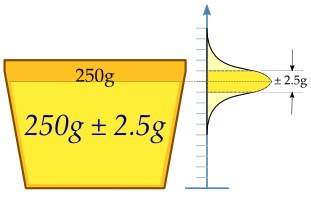
A machine fills cups with a liquid, and is supposed to be adjusted so that the content of the cups is 250 g of liquid. As the machine cannot fill every cup with exactly 250.0 g, the content added to individual cups shows some variation, and is considered a random variable X. This variation is assumed to be normally distributed around the desired average of 250 g, with a standard deviation, σ, of 2.5 g. To determine if the machine is adequately calibrated, a sample of n = 25 cups of liquid is chosen at random and the cups are weighed. The resulting measured masses of liquid are X₁, ..., X₂₅, a random sample from X.

To get an impression of the expectation μ, it is sufficient to give an estimate. The appropriate estimator is the sample mean:

${\displaystyle {\hat {\mu }}={\bar {X}}={\frac {1}{n}}\sum _{i=1}^{n}X_{i}.}$

The sample shows actual weights x₁, ..., x₂₅, with mean:

${\displaystyle {\bar {x}}={\frac {1}{25}}\sum _{i=1}^{25}x_{i}=250.2{\text{ grams}}.}$

If we take another sample of 25 cups, we could easily expect to find mean values like 250.4 or 251.1 grams. A sample mean value of 280 grams however would be extremely rare if the mean content of the cups is in fact close to 250 grams. There is a whole interval around the observed value 250.2 grams of the sample mean within which, if the whole population mean actually takes a value in this range, the observed data would not be considered particularly unusual. Such an interval is called a confidence interval for the parameter μ. How do we calculate such an interval? The endpoints of the interval have to be calculated from the sample, so they are statistics, functions of the sample X₁, ..., X₂₅ and hence random variables themselves.

In our case we may determine the endpoints by considering that the sample mean X from a normally distributed sample is also normally distributed, with the same expectation μ, but with a standard error of:

${\displaystyle {\frac {\sigma }{\sqrt {n}}}={\frac {2.5{\text{ g}}}{\sqrt {25}}}=0.5{\text{ grams}}}$

By standardizing, we get a random variable:

${\displaystyle Z={\frac {{\bar {X}}-\mu }{\sigma /{\sqrt {n}}}}={\frac {{\bar {X}}-\mu }{0.5}}}$

dependent on the parameter μ to be estimated, but with a standard normal distribution independent of the parameter μ. Hence it is possible to find numbers −z and z, independent of μ, between which Z lies with probability 1 − α, a measure of how confident we want to be.

We take 1 − α = 0.95, for example. So we have:

${\displaystyle P(-z\leq Z\leq z)=1-\alpha =0.95.}$

The number z follows from the cumulative distribution function, in this case the cumulative normal distribution function:

${\displaystyle {\begin{aligned}\Phi (z)&=P(Z\leq z)=1-{\tfrac {\alpha }{2}}=0.975,\\[6pt]z&=\Phi ^{-1}(\Phi (z))=\Phi ^{-1}(0.975)=1.96,\end{aligned}}}$

and we get:

${\displaystyle {\begin{aligned}0.95&=1-\alpha =P(-z\leq Z\leq z)=P\left(-1.96\leq {\frac {{\bar {X}}-\mu }{\sigma /{\sqrt {n}}}}\leq 1.96\right)\\[6pt]&=P\left({\bar {X}}-1.96{\frac {\sigma }{\sqrt {n}}}\leq \mu \leq {\bar {X}}+1.96{\frac {\sigma }{\sqrt {n}}}\right).\end{aligned}}}$

In other words, the lower endpoint of the 95% confidence interval is:

${\displaystyle {\text{Lower endpoint}}={\bar {X}}-1.96{\frac {\sigma }{\sqrt {n}}},}$

and the upper endpoint of the 95% confidence interval is:

${\displaystyle {\text{Upper endpoint}}={\bar {X}}+1.96{\frac {\sigma }{\sqrt {n}}}.}$

With the values in this example, the confidence interval is:

${\displaystyle {\begin{aligned}0.95&=\Pr({\bar {X}}-1.96\times 0.5\leq \mu \leq {\bar {X}}+1.96\times 0.5)\\[6pt]&=\Pr({\bar {X}}-0.98\leq \mu \leq {\bar {X}}+0.98).\end{aligned}}}$

As the standard deviation of the population σ is known in this case, the distribution of the sample mean ${\displaystyle {\bar {X}}}$ is a normal distribution with ${\displaystyle \mu }$ the only unknown parameter. In the theoretical example below, the parameter σ is also unknown, which calls for using the Student's t-distribution.

This might be interpreted as: with probability 0.95 we will find a confidence interval in which the value of parameter μ will be between the stochastic endpoints

${\displaystyle \!{\bar {X}}-0{.}98}$

and

${\displaystyle \!{\bar {X}}+0.98.}$

This does not mean there is 0.95 probability that the value of parameter μ is in the interval obtained by using the currently computed value of the sample mean,

${\displaystyle ({\bar {x}}-0.98,\,{\bar {x}}+0.98).}$

Instead, every time the measurements are repeated, there will be another value for the mean X of the sample. In 95% of the cases μ will be between the endpoints calculated from this mean, but in 5% of the cases it will not be. The actual confidence interval is calculated by entering the measured masses in the formula. Our 0.95 confidence interval becomes:

${\displaystyle ({\bar {x}}-0.98;{\bar {x}}+0.98)=(250.2-0.98;250.2+0.98)=(249.22;251.18).\,}$

The blue vertical line segments represent 50 realizations of a confidence interval for the population mean μ, represented as a red horizontal dashed line; note that some confidence intervals do not contain the population mean, as expected.

In other words, the 95% confidence interval is between the lower endpoint 249.22 g and the upper endpoint 251.18 g.

As the desired value 250 of μ is within the resulted confidence interval, there is no reason to believe the machine is wrongly calibrated.

The calculated interval has fixed endpoints, where μ might be in between (or not). Thus this event has probability either 0 or 1. One cannot say: "with probability (1 − α) the parameter μ lies in the confidence interval." One only knows that by repetition in 100(1 − α)% of the cases, μ will be in the calculated interval. In 100α% of the cases however it does not. And unfortunately one does not know in which of the cases this happens. That is (instead of using the term "probability") why one can say: "with confidence level 100(1 − α) %, μ lies in the confidence interval."

The maximum error is calculated to be 0.98 since it is the difference between the value that we are confident of with upper or lower endpoint.

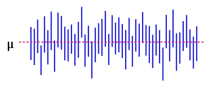
The figure on the right shows 50 realizations of a confidence interval for a given population mean μ. If we randomly choose one realization, the probability is 95% we end up having chosen an interval that contains the parameter; however, we may be unlucky and have picked the wrong one. We will never know; we are stuck with our interval.

Medical research often estimates the effects of an intervention or exposure in a certain population.[34] Usually, researchers have determined the significance of the effects based on the p-value; however, recently there has been a push for more statistical information in order to provide a stronger basis for the estimations.[34] One way to resolve this issue is also requiring the reporting of the confidence interval. Below are two examples of how confidence intervals are used and reported for research:

In a 2004 study, Briton and colleagues conducted a study on evaluating relation of infertility to ovarian cancer. The incidence ratio of 1.98 was reported for a 95% Confidence (CI) interval with a ratio range of 1.4 to 2.6.[35] The statistic was reported as the following in the paper: “(standardized incidence ratio = 1.98; 95% CI, 1.4–2.6).”[35] This means that, based on the sample studied, infertile females have an ovarian cancer incidence that is 1.98 times higher than non-infertile females. Furthermore, it also means that we are 95% confident that the true incidence ratio in all the infertile female population lies in the range from 1.4 to 2.6.[35] Therefore, there is a 5% probability that the true incidence ratio may lie out of the range of 1.4 to 2.6 values.[35] Overall, the confidence interval provided more statistical information in that it reported the lowest and largest effects that are likely to occur for the studied variable while still providing information on the significance of the effects observed.[34]

In a 2018 study, the prevalence and disease burden of atopic dermatitis in the US Adult Population was understood with the use of 95% confidence intervals.[36] It was reported that among 1,278 participating adults, the prevalence of atopic dermatitis was 7.3% (5.9–8.8).[36] Furthermore, 60.1% (56.1–64.1) of participants were classified to have mild atopic dermatitis while 28.9% (25.3–32.7) had moderate and 11% (8.6–13.7) had severe.[36] The study confirmed that there is a high prevalence and disease burden of atopic dermatitis in the population.

Suppose {X₁, ..., X_n} is an independent sample from a normally distributed population with unknown (parameters) mean μ and variance σ². Let

${\displaystyle {\bar {X}}=(X_{1}+\cdots +X_{n})/n\,,}$

${\displaystyle S^{2}={\frac {1}{n-1}}\sum _{i=1}^{n}(X_{i}-{\bar {X}}\,)^{2}.}$

Where X is the sample mean, and S² is the sample variance. Then

${\displaystyle T={\frac {{\bar {X}}-\mu }{S/{\sqrt {n}}}}}$

has a Student's t-distribution with n − 1 degrees of freedom.[37] Note that the distribution of T does not depend on the values of the unobservable parameters μ and σ²; i.e., it is a pivotal quantity. Suppose we wanted to calculate a 95% confidence interval for μ. Then, denoting c as the 97.5th percentile of this distribution,

${\displaystyle \Pr(-c\leq T\leq c)=0.95\,}$

Note that "97.5th" and "0.95" are correct in the preceding expressions. There is a 2.5% chance that ${\displaystyle T}$ will be less than ${\displaystyle -}$${\displaystyle c}$ and a 2.5% chance that it will be larger than ${\displaystyle +}$${\displaystyle c}$. Thus, the probability that ${\displaystyle T}$ will be between ${\displaystyle -}$${\displaystyle c}$ and ${\displaystyle +}$${\displaystyle c}$ is 95%.

Consequently,

${\displaystyle \Pr \left({\bar {X}}-{\frac {cS}{\sqrt {n}}}\leq \mu \leq {\bar {X}}+{\frac {cS}{\sqrt {n}}}\right)=0.95\,}$

and we have a theoretical (stochastic) 95% confidence interval for μ.

After observing the sample we find values x for X and s for S, from which we compute the confidence interval

${\displaystyle \left[{\bar {x}}-{\frac {cs}{\sqrt {n}}},{\bar {x}}+{\frac {cs}{\sqrt {n}}}\right],\,}$

an interval with fixed numbers as endpoints, of which we can no longer say there is a certain probability it contains the parameter μ; either μ is in this interval or isn't.

A prediction interval for a random variable is defined similarly to a confidence interval for a statistical parameter. Consider an additional random variable Y which may or may not be statistically dependent on the random sample X. Then (u(X), v(X)) provides a prediction interval for the as-yet-to-be observed value y of Y if

${\displaystyle {\Pr }_{\theta ,\varphi }(u(X)<Y<v(X))=\gamma {\text{ for all }}(\theta ,\varphi ).\,}$

Here Pr_θ,φ indicates the joint probability distribution of the random variables (X, Y), where this distribution depends on the statistical parameters (θ, φ).

A Bayesian interval estimate is called a credible interval. Using much of the same notation as above, the definition of a credible interval for the unknown true value of θ is, for a given γ,[38]

${\displaystyle \Pr(u(x)<\Theta <v(x)\mid X=x)=\gamma .\,}$

Here Θ is used to emphasize that the unknown value of θ is being treated as a random variable. The definitions of the two types of intervals may be compared as follows.

• The definition of a confidence interval involves probabilities calculated from the distribution of X for a given (θ, φ) (or conditional on these values) and the condition needs to hold for all values of (θ, φ).
• The definition of a credible interval involves probabilities calculated from the distribution of Θ conditional on the observed values of X = x and marginalised (or averaged) over the values of Φ, where this last quantity is the random variable corresponding to the uncertainty about the nuisance parameters in φ.

Note that the treatment of the nuisance parameters above is often omitted from discussions comparing confidence and credible intervals but it is markedly different between the two cases.

In some simple standard cases, the intervals produced as confidence and credible intervals from the same data set can be identical. They are very different if informative prior information is included in the Bayesian analysis, and may be very different for some parts of the space of possible data even if the Bayesian prior is relatively uninformative.

There is disagreement about which of these methods produces the most useful results: the mathematics of the computations are rarely in question–confidence intervals being based on sampling distributions, credible intervals being based on Bayes' theorem–but the application of these methods, the utility and interpretation of the produced statistics, is debated.

An approximate confidence interval for a population mean can be constructed for random variables that are not normally distributed in the population, relying on the central limit theorem, if the sample sizes and counts are big enough. The formulae are identical to the case above (where the sample mean is actually normally distributed about the population mean). The approximation will be quite good with only a few dozen observations in the sample if the probability distribution of the random variable is not too different from the normal distribution (e.g. its cumulative distribution function does not have any discontinuities and its skewness is moderate).

One type of sample mean is the mean of an indicator variable, which takes on the value 1 for true and the value 0 for false. The mean of such a variable is equal to the proportion that has the variable equal to one (both in the population and in any sample). This is a useful property of indicator variables, especially for hypothesis testing. To apply the central limit theorem, one must use a large enough sample. A rough rule of thumb is that one should see at least 5 cases in which the indicator is 1 and at least 5 in which it is 0. Confidence intervals constructed using the above formulae may include negative numbers or numbers greater than 1, but proportions obviously cannot be negative or exceed 1. Additionally, sample proportions can only take on a finite number of values, so the central limit theorem and the normal distribution are not the best tools for building a confidence interval. See "Binomial proportion confidence interval" for better methods which are specific to this case.

Since confidence interval theory was proposed, a number of counter-examples to the theory have been developed to show how the interpretation of confidence intervals can be problematic, at least if one interprets them naïvely.

Welch[39] presented an example which clearly shows the difference between the theory of confidence intervals and other theories of interval estimation (including Fisher's fiducial intervals and objective Bayesian intervals). Robinson[40] called this example "[p]ossibly the best known counterexample for Neyman's version of confidence interval theory." To Welch, it showed the superiority of confidence interval theory; to critics of the theory, it shows a deficiency. Here we present a simplified version.

Suppose that ${\displaystyle X_{1},X_{2}}$ are independent observations from a Uniform(θ − 1/2, θ + 1/2) distribution. Then the optimal 50% confidence procedure[41] is

${\displaystyle {\bar {X}}\pm {\begin{cases}{\dfrac {|X_{1}-X_{2}|}{2}}&{\text{if }}|X_{1}-X_{2}|<1/2\\[8pt]{\dfrac {1-|X_{1}-X_{2}|}{2}}&{\text{if }}|X_{1}-X_{2}|\geq 1/2.\end{cases}}}$

A fiducial or objective Bayesian argument can be used to derive the interval estimate

${\displaystyle {\bar {X}}\pm {\frac {1-|X_{1}-X_{2}|}{4}},}$

which is also a 50% confidence procedure. Welch showed that the first confidence procedure dominates the second, according to desiderata from confidence interval theory; for every ${\displaystyle \theta _{1}\neq \theta }$, the probability that the first procedure contains ${\displaystyle \theta _{1}}$ is less than or equal to the probability that the second procedure contains ${\displaystyle \theta _{1}}$. The average width of the intervals from the first procedure is less than that of the second. Hence, the first procedure is preferred under classical confidence interval theory.

However, when ${\displaystyle |X_{1}-X_{2}|\geq 1/2}$, intervals from the first procedure are guaranteed to contain the true value ${\displaystyle \theta }$: Therefore, the nominal 50% confidence coefficient is unrelated to the uncertainty we should have that a specific interval contains the true value. The second procedure does not have this property.

Moreover, when the first procedure generates a very short interval, this indicates that ${\displaystyle X_{1},X_{2}}$ are very close together and hence only offer the information in a single data point. Yet the first interval will exclude almost all reasonable values of the parameter due to its short width. The second procedure does not have this property.

The two counter-intuitive properties of the first procedure—100% coverage when ${\displaystyle X_{1},X_{2}}$ are far apart and almost 0% coverage when ${\displaystyle X_{1},X_{2}}$ are close together—balance out to yield 50% coverage on average. However, despite the first procedure being optimal, its intervals offer neither an assessment of the precision of the estimate nor an assessment of the uncertainty one should have that the interval contains the true value.

This counter-example is used to argue against naïve interpretations of confidence intervals. If a confidence procedure is asserted to have properties beyond that of the nominal coverage (such as relation to precision, or a relationship with Bayesian inference), those properties must be proved; they do not follow from the fact that a procedure is a confidence procedure.

Steiger[42] suggested a number of confidence procedures for common effect size measures in ANOVA. Morey et al.[13] point out that several of these confidence procedures, including the one for ω², have the property that as the F statistic becomes increasingly small—indicating misfit with all possible values of ω²—the confidence interval shrinks and can even contain only the single value ω² = 0; that is, the CI is infinitesimally narrow (this occurs when ${\displaystyle p\geq 1-\alpha /2}$ for a ${\displaystyle 100(1-\alpha )\%}$ CI).

This behavior is consistent with the relationship between the confidence procedure and significance testing: as F becomes so small that the group means are much closer together than we would expect by chance, a significance test might indicate rejection for most or all values of ω². Hence the interval will be very narrow or even empty (or, by a convention suggested by Steiger, containing only 0). However, this does not indicate that the estimate of ω² is very precise. In a sense, it indicates the opposite: that the trustworthiness of the results themselves may be in doubt. This is contrary to the common interpretation of confidence intervals that they reveal the precision of the estimate.

• Confidence interval for binomial distribution
• Confidence interval for exponent of the power law distribution
• Confidence interval for mean of the exponential distribution
• Confidence interval for mean of the Poisson distribution
• Confidence intervals for mean and variance of the normal distribution

Wikimedia Commons has media related to Confidence interval.

• The Exploratory Software for Confidence Intervals tutorial programs that run under Excel
• Confidence interval calculators for R-Squares, Regression Coefficients, and Regression Intercepts
• Weisstein, Eric W. "Confidence Interval". MathWorld.
• CAUSEweb.org Many resources for teaching statistics including Confidence Intervals.
• An interactive introduction to Confidence Intervals
• Confidence Intervals: Confidence Level, Sample Size, and Margin of Error by Eric Schulz, the Wolfram Demonstrations Project.
• Confidence Intervals in Public Health. Straightforward description with examples and what to do about small sample sizes or rates near 0.

• GraphPad QuickCalcs
• TAMU's Confidence Interval Calculators
• MBAStats confidence interval and hypothesis test calculators
• Stats Journal – statistics calculator online

References

- Dekking, F.M. (Frederik Michel), 1946- (2005). A modern introduction to probability and statistics : understanding why and how. Springer. ISBN 1-85233-896-2. OCLC 783259968.CS1 maint: multiple names: authors list (link)
- Cox D.R., Hinkley D.V. (1974) Theoretical Statistics, Chapman & Hall, p49, p209
- Kendall, M.G. and Stuart, D.G. (1973) The Advanced Theory of Statistics. Vol 2: Inference and Relationship, Griffin, London. Section 20.4
- Neyman, J. (1937). "Outline of a Theory of Statistical Estimation Based on the Classical Theory of Probability". Philosophical Transactions of the Royal Society A. 236 (767): 333–380. Bibcode:1937RSPTA.236..333N. doi:10.1098/rsta.1937.0005. JSTOR 91337.
- Illowsky, Barbara. Introductory statistics. Dean, Susan L., 1945-, Illowsky, Barbara., OpenStax College. Houston, Texas. ISBN 978-1-947172-05-0. OCLC 899241574.
- Zar, Jerrold H. (199). Biostatistical Analysis (4th ed.). Upper Saddle River, N.J.: Prentice Hall. pp. 43–45. ISBN 978-0130815422. OCLC 39498633.
- Cox D.R., Hinkley D.V. (1974) Theoretical Statistics, Chapman & Hall, pp 214, 225, 233
- "Archived copy" (PDF). Archived from the original (PDF) on 2016-03-04. Retrieved 2014-09-16.CS1 maint: archived copy as title (link)
- Hoekstra, R., R. D. Morey, J. N. Rouder, and E-J. Wagenmakers, 2014. Robust misinterpretation of confidence intervals. Psychonomic Bulletin Review, in press.
- Scientists’ grasp of confidence intervals doesn’t inspire confidence, Science News, July 3, 2014
- Greenland, Sander; Senn, Stephen J.; Rothman, Kenneth J.; Carlin, John B.; Poole, Charles; Goodman, Steven N.; Altman, Douglas G. (April 2016). "Statistical tests, P values, confidence intervals, and power: a guide to misinterpretations". European Journal of Epidemiology. 31 (4): 337–350. doi:10.1007/s10654-016-0149-3. ISSN 0393-2990. PMC 4877414. PMID 27209009.
- Morey, R. D.; Hoekstra, R.; Rouder, J. N.; Lee, M. D.; Wagenmakers, E.-J. (2016). "The Fallacy of Placing Confidence in Confidence Intervals". Psychonomic Bulletin & Review. 23 (1): 103–123. doi:10.3758/s13423-015-0947-8. PMC 4742505. PMID 26450628.
- "1.3.5.2. Confidence Limits for the Mean". nist.gov. Archived from the original on 2008-02-05. Retrieved 2014-09-16.
- Mayo, D. G. (1981) "In defence of the Neyman–Pearson theory of confidence intervals", Philosophy of Science, 48 (2), 269–280. JSTOR 187185
- Sandercock, Peter A.G. (May 2015). "Short History of Confidence Intervals". American Heart Association.
- T. Seidenfeld, Philosophical Problems of Statistical Inference: Learning from R.A. Fisher, Springer-Verlag, 1979
- "Statistical significance defined using the five sigma standard".
- Cox D.R., Hinkley D.V. (1974) Theoretical Statistics, Chapman & Hall, Section 7.2(iii)
- Pav Kalinowski, "Understanding Confidence Intervals (CIs) and Effect Size Estimation", Observer Vol.23, No.4 April 2010.
- Andrea Knezevic, "Overlapping Confidence Intervals and Statistical Significance", StatNews # 73: Cornell Statistical Consulting Unit, October 2008.
- Goldstein, H.; Healey, M.J.R. (1995). "The graphical presentation of a collection of means". Journal of the Royal Statistical Society. 158 (1): 175–77. CiteSeerX 10.1.1.649.5259. doi:10.2307/2983411. JSTOR 2983411.
- Wolfe R, Hanley J (Jan 2002). "If we're so different, why do we keep overlapping? When 1 plus 1 doesn't make 2". CMAJ. 166 (1): 65–6. PMC 99228. PMID 11800251.
- Daniel Smith, "Overlapping confidence intervals are not a statistical test Archived 2016-02-22 at the Wayback Machine", California Dept of Health Services, 26th Annual Institute on Research and Statistics, Sacramento, CA, March, 2005.
- p.65 in W. Härdle, M. Müller, S. Sperlich, A. Werwatz (2004), Nonparametric and Semiparametric Models, Springer, ISBN 3-540-20722-8
- "Checking Out Statistical Confidence Interval Critical Values – For Dummies". www.dummies.com. Retrieved 2016-02-11.
- "Confidence Intervals". www.stat.yale.edu. Retrieved 2016-02-11.
- "Confidence Intervals with the z and t-distributions | Jacob Montgomery". pages.wustl.edu. Retrieved 2019-12-14.
- Probability & statistics for engineers & scientists. Walpole, Ronald E., Myers, Raymond H., Myers, Sharon L., 1944-, Ye, Keying. (9th ed.). Boston: Prentice Hall. 2012. ISBN 978-0-321-62911-1. OCLC 537294244.CS1 maint: others (link)
- George G. Roussas (1997) A Course in Mathematical Statistics, 2nd Edition, Academic Press, p397
- Cox D.R., Hinkley D.V. (1974) Theoretical Statistics, Chapman & Hall, p. 210
- Abramovich, Felix, and Ya'acov Ritov. Statistical Theory: A Concise Introduction. CRC Press, 2013. Pages 121–122
- Attia, Abdelhamid (December 2005). "Evidence-based Medicine Corner- Why should researchers report the confidence interval in modern research?". Middle East Fertility Society Journal. 10.
- Brinton, Louise A; Lamb, Emmet J; Moghissi, Kamran S; Scoccia, Bert; Althuis, Michelle D; Mabie, Jerome E; Westhoff, Carolyn L (August 2004). "Ovarian cancer risk associated with varying causes of infertility". Fertility and Sterility. 82 (2): 405–414. doi:10.1016/j.fertnstert.2004.02.109. ISSN 0015-0282. PMID 15302291.
- Chiesa Fuxench, Zelma C.; Block, Julie K.; Boguniewicz, Mark; Boyle, John; Fonacier, Luz; Gelfand, Joel M.; Grayson, Mitchell H.; Margolis, David J.; Mitchell, Lynda; Silverberg, Jonathan I.; Schwartz, Lawrence (March 2019). "Atopic Dermatitis in America Study: A Cross-Sectional Study Examining the Prevalence and Disease Burden of Atopic Dermatitis in the US Adult Population". The Journal of Investigative Dermatology. 139 (3): 583–590. doi:10.1016/j.jid.2018.08.028. ISSN 1523-1747. PMID 30389491. no-break space character in
Bibliography

- Fisher, R.A. (1956) Statistical Methods and Scientific Inference. Oliver and Boyd, Edinburgh. (See p. 32.)
- Freund, J.E. (1962) Mathematical Statistics Prentice Hall, Englewood Cliffs, NJ. (See pp. 227–228.)
- Hacking, I. (1965) Logic of Statistical Inference. Cambridge University Press, Cambridge. ISBN 0-521-05165-7
- Keeping, E.S. (1962) Introduction to Statistical Inference. D. Van Nostrand, Princeton, NJ.
- Kiefer, J. (1977). "Conditional Confidence Statements and Confidence Estimators (with discussion)". Journal of the American Statistical Association. 72 (360a): 789–827. doi:10.1080/01621459.1977.10479956. JSTOR 2286460.
- Neyman, J. (1937) "Outline of a Theory of Statistical Estimation Based on the Classical Theory of Probability" Philosophical Transactions of the Royal Society of London A, 236, 333–380. (Seminal work.)
- Robinson, G.K. (1975). "Some Counterexamples to the Theory of Confidence Intervals". Biometrika. 62 (1): 155–161. doi:10.1093/biomet/62.1.155. JSTOR 2334498.
- Savage, L. J. (1962), The Foundations of Statistical Inference. Methuen, London.
- Smithson, M. (2003) Confidence intervals. Quantitative Applications in the Social Sciences Series, No. 140. Belmont, CA: SAGE Publications. ISBN 978-0-7619-2499-9.
- Mehta, S. (2014) Statistics Topics ISBN 978-1-4992-7353-3
- Hazewinkel, Michiel, ed. (2001) [1994], "Confidence estimation", Encyclopedia of Mathematics, Springer Science+Business Media B.V. / Kluwer Academic Publishers, ISBN 978-1-55608-010-4
- Morey, R. D.; Hoekstra, R.; Rouder, J. N.; Lee, M. D.; Wagenmakers, E.-J. (2016). "The fallacy of placing confidence in confidence intervals". Psychonomic Bulletin & Review. 23 (1): 103–123. doi:10.3758/s13423-015-0947-8. PMC 4742505. PMID 26450628.
External links