Breadth-first search
Breadth-first search (BFS) is an algorithm for traversing or searching tree or graph data structures. It starts at the tree root (or some arbitrary node of a graph, sometimes referred to as a 'search key'[1]), and explores all of the neighbor nodes at the present depth prior to moving on to the nodes at the next depth level.
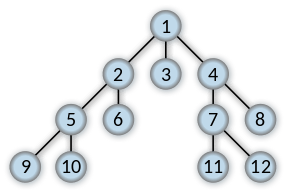 Order in which the nodes get expanded Order in which the nodes are expanded | |
| Class | Search algorithm |
|---|---|
| Data structure | Graph |
| Worst-case performance | |
| Worst-case space complexity | |


| Graph and tree search algorithms |
|---|
| Listings |
|
| Related topics |
|
It uses the opposite strategy as depth-first search, which instead explores the node branch as far as possible before being forced to backtrack and expand other nodes.[2]
BFS and its application in finding connected components of graphs were invented in 1945 by Konrad Zuse, in his (rejected) Ph.D. thesis on the Plankalkül programming language, but this was not published until 1972.[3] It was reinvented in 1959 by Edward F. Moore, who used it to find the shortest path out of a maze,[4][5] and later developed by C. Y. Lee into a wire routing algorithm (published 1961).[6]
Pseudocode
Input: A graph Graph and a starting vertex root of Graph
Output: Goal state. The parent links trace the shortest path back to root
1  procedure BFS(G, start_v) is
2      let Q be a queue
3      label start_v as discovered
4      Q.enqueue(start_v)
5      while Q is not empty do
6          v := Q.dequeue()
7          if v is the goal then
8              return v
9          for all edges from v to w in G.adjacentEdges(v) do
10             if w is not labeled as discovered then
11                 label w as discovered
12                 w.parent := v
13                 Q.enqueue(w)
More details
This non-recursive implementation is similar to the non-recursive implementation of depth-first search, but differs from it in two ways:
- it uses a queue (First In First Out) instead of a stack and
- it checks whether a vertex has been discovered before enqueueing the vertex rather than delaying this check until the vertex is dequeued from the queue.
The Q queue contains the frontier along which the algorithm is currently searching.
Nodes can be labelled as discovered by storing them in a set, or by an attribute on each node, depending on the implementation.
Note that the word node is usually interchangeable with the word vertex.
The parent attribute of each node is useful for accessing the nodes in a shortest path, for example by backtracking from the destination node up to the starting node, once the BFS has been run, and the predecessors nodes have been set.
Breadth-first search produces a so-called breadth first tree. You can see how a breadth first tree looks in the following example.


Analysis
Time and space complexity
The time complexity can be expressed as , since every vertex and every edge will be explored in the worst case. is the number of vertices and is the number of edges in the graph. Note that may vary between and , depending on how sparse the input graph is.[7]


When the number of vertices in the graph is known ahead of time, and additional data structures are used to determine which vertices have already been added to the queue, the space complexity can be expressed as , where is the cardinality of the set of vertices. This is in addition to the space required for the graph itself, which may vary depending on the graph representation used by an implementation of the algorithm.

When working with graphs that are too large to store explicitly (or infinite), it is more practical to describe the complexity of breadth-first search in different terms: to find the nodes that are at distance d from the start node (measured in number of edge traversals), BFS takes O(bd + 1) time and memory, where b is the "branching factor" of the graph (the average out-degree).[8]:81
Completeness
In the analysis of algorithms, the input to breadth-first search is assumed to be a finite graph, represented explicitly as an adjacency list or similar representation. However, in the application of graph traversal methods in artificial intelligence the input may be an implicit representation of an infinite graph. In this context, a search method is described as being complete if it is guaranteed to find a goal state if one exists. Breadth-first search is complete, but depth-first search is not. When applied to infinite graphs represented implicitly, breadth-first search will eventually find the goal state, but depth-first search may get lost in parts of the graph that have no goal state and never return.[9]
BFS ordering
An enumeration of the vertices of a graph is said to be a BFS ordering if it is the possible output of the application of BFS to this graph.
Let be a graph with vertices. Recall that is the set of neighbors of . For be a list of distinct elements of , for , let be the least such that is a neighbor of , if such a exists, and be otherwise.


Let be an enumeration of the vertices of . The enumeration is said to be a BFS ordering (with source ) if, for all , is the vertex such that is minimal. Equivalently, is a BFS ordering if, for all with , there exists a neighbor of such that .


Applications
Breadth-first search can be used to solve many problems in graph theory, for example:
- Copying garbage collection, Cheney's algorithm
- Finding the shortest path between two nodes u and v, with path length measured by number of edges (an advantage over depth-first search)[10]
- (Reverse) Cuthill–McKee mesh numbering
- Ford–Fulkerson method for computing the maximum flow in a flow network
- Serialization/Deserialization of a binary tree vs serialization in sorted order, allows the tree to be re-constructed in an efficient manner.
- Construction of the failure function of the Aho-Corasick pattern matcher.
- Testing bipartiteness of a graph.
See also
- Depth-first search
- Iterative deepening depth-first search
- Level structure
- Lexicographic breadth-first search
- Parallel breadth-first search
References
- "Graph500 benchmark specification (supercomputer performance evaluation)". Graph500.org, 2010. Archived from the original on 2015-03-26. Retrieved 2015-03-15.
- Cormen Thomas H.; et al. (2009). "22.3". Introduction to Algorithms. MIT Press.
- Zuse, Konrad (1972), Der Plankalkül (in German), Konrad Zuse Internet Archive. See pp. 96–105 of the linked pdf file (internal numbering 2.47–2.56).
- Moore, Edward F. (1959). "The shortest path through a maze". Proceedings of the International Symposium on the Theory of Switching. Harvard University Press. pp. 285–292. As cited by Cormen, Leiserson, Rivest, and Stein.
- Skiena, Steven (2008). "Sorting and Searching". The Algorithm Design Manual. Springer. p. 480. Bibcode:2008adm..book.....S. doi:10.1007/978-1-84800-070-4_4. ISBN 978-1-84800-069-8.
- Lee, C. Y. (1961). "An Algorithm for Path Connections and Its Applications". IRE Transactions on Electronic Computers. doi:10.1109/TEC.1961.5219222.
- Cormen, Thomas H.; Leiserson, Charles E.; Rivest, Ronald L.; Stein, Clifford (2001) [1990]. "22.2 Breadth-first search". Introduction to Algorithms (2nd ed.). MIT Press and McGraw-Hill. pp. 531–539. ISBN 0-262-03293-7.
- Russell, Stuart; Norvig, Peter (2003) [1995]. Artificial Intelligence: A Modern Approach (2nd ed.). Prentice Hall. ISBN 978-0137903955.
- Coppin, B. (2004). Artificial intelligence illuminated. Jones & Bartlett Learning. pp. 79–80.
- Aziz, Adnan; Prakash, Amit (2010). "4. Algorithms on Graphs". Algorithms for Interviews. p. 144. ISBN 978-1453792995.
- Knuth, Donald E. (1997), The Art of Computer Programming Vol 1. 3rd ed., Boston: Addison-Wesley, ISBN 978-0-201-89683-1
External links
| Wikimedia Commons has media related to Breadth-first search. |