Traffic flow
In mathematics and transportation engineering, traffic flow is the study of interactions between travellers (including pedestrians, cyclists, drivers, and their vehicles) and infrastructure (including highways, signage, and traffic control devices), with the aim of understanding and developing an optimal transport network with efficient movement of traffic and minimal traffic congestion problems.
History
Attempts to produce a mathematical theory of traffic flow date back to the 1920s, when Frank Knight first produced an analysis of traffic equilibrium, which was refined into Wardrop's first and second principles of equilibrium in 1952.
Nonetheless, even with the advent of significant computer processing power, to date there has been no satisfactory general theory that can be consistently applied to real flow conditions. Current traffic models use a mixture of empirical and theoretical techniques. These models are then developed into traffic forecasts, and take account of proposed local or major changes, such as increased vehicle use, changes in land use or changes in mode of transport (with people moving from bus to train or car, for example), and to identify areas of congestion where the network needs to be adjusted.
Overview
Traffic behaves in a complex and nonlinear way, depending on the interactions of a large number of vehicles. Due to the individual reactions of human drivers, vehicles do not interact simply following the laws of mechanics, but rather display cluster formation and shock wave propagation, both forward and backward, depending on vehicle density. Some mathematical models of traffic flow use a vertical queue assumption, in which the vehicles along a congested link do not spill back along the length of the link.
In a free-flowing network, traffic flow theory refers to the traffic stream variables of speed, flow, and concentration. These relationships are mainly concerned with uninterrupted traffic flow, primarily found on freeways or expressways.[1] Flow conditions are considered "free" when less than 12 vehicles per mile per lane are on a road. "Stable" is sometimes described as 12–30 vehicles per mile per lane. As the density reaches the maximum mass flow rate (or flux) and exceeds the optimum density (above 30 vehicles per mile per lane), traffic flow becomes unstable, and even a minor incident can result in persistent stop-and-go driving conditions. A "breakdown" condition occurs when traffic becomes unstable and exceeds 67 vehicles per mile per lane.[2] "Jam density" refers to extreme traffic density when traffic flow stops completely, usually in the range of 185–250 vehicles per mile per lane.[3]
However, calculations about congested networks are more complex and rely more on empirical studies and extrapolations from actual road counts. Because these are often urban or suburban in nature, other factors (such as road-user safety and environmental considerations) also influence the optimum conditions.
There are common spatiotemporal empirical features of traffic congestion that are qualitatively the same for different highways in different countries, measured during years of traffic observations. Some of these common features of traffic congestion define synchronized flow and wide moving jam traffic phases of congested traffic in Kerner’s three-phase traffic theory of traffic flow (see also Traffic congestion reconstruction with Kerner’s three-phase theory).
Single vehicle dynamics
Motion as a function of time
Let be the vehicle trajectory. Then,


Or, equivalently,

where all the variables with subscript "0" are given initial conditions at time .

Motion as a function of distance
In some applications it is convenient to take distance as the independent variable. A vehicle trajectory is represented by , the inverse function of .

- If is given, can be derived as: .
- If is given, can be derived using the chain rule: , or . This can also be written as , or better as , which can be integrated to give . Hence,


Motion as a function of speed
Vehicle kinematics models give the "desired acceleration" that the driver imposes to the vehicle when traveling at a speed at time under free-flow conditions. A desired acceleration model captures both driver behavior and the physical limitations imposed by roadway geometry on the engine.


Noting that we have , which by integration gives . The position can be derived using the chain rule:


This gives and hence


Linear acceleration model and dimensionless formulation
For light vehicles, a good approximation is a linearly decreasing function of the speed:

where has units of and can be interpreted as a desired speed. The reasonable typical value[4] of is 0.06.


Dimensionless formulations are convenient because they reduce the number of parameters involved in a problem. Define,which means that we measure time in units of , and the speed in units of . The quantity


is the time scale of the problem. This means that the time for the system to reach equilibrium from a perturbation is comparable to .

The corresponding transformation for the space variable

is obtained by a change of variable noting that

The linear acceleration model is now

with the initial condition . Setting the equations of motion become


and the only parameter is the initial condition .

A completely parameter-free formulation is given by the transformation

The acceleration model becomes with initial condition ; this gives


Traffic stream properties
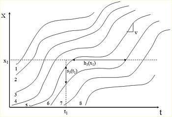
Traffic flow is generally constrained along a one-dimensional pathway (e.g. a travel lane). A time-space diagram shows graphically the flow of vehicles along a pathway over time. Time is displayed along the horizontal axis, and distance is shown along the vertical axis. Traffic flow in a time-space diagram is represented by the individual trajectory lines of individual vehicles. Vehicles following each other along a given travel lane will have parallel trajectories, and trajectories will cross when one vehicle passes another. Time-space diagrams are useful tools for displaying and analyzing the traffic flow characteristics of a given roadway segment over time (e.g. analyzing traffic flow congestion).
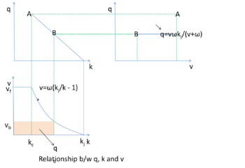
There are three main variables to visualize a traffic stream: speed (v), density (indicated k; the number of vehicles per unit of space), and flow (indicated q; the number of vehicles per unit of time).
Speed
Speed is the distance covered per unit time. One cannot track the speed of every vehicle; so, in practice, average speed is measured by sampling vehicles in a given area over a period of time. Two definitions of average speed are identified: "time mean speed" and "space mean speed".
- "Time mean speed" is measured at a reference point on the roadway over a period of time. In practice, it is measured by the use of loop detectors. Loop detectors, when spread over a reference area, can identify each vehicle and can track its speed. However, average speed measurements obtained from this method are not accurate because instantaneous speeds averaged over several vehicles do not account for the difference in travel time for the vehicles that are traveling at different speeds over the same distance.

where m represents the number of vehicles passing the fixed point and vi is the speed of the ith vehicle.
- "Space mean speed" is measured over the whole roadway segment. Consecutive pictures or video of a roadway segment track the speed of individual vehicles, and then the average speed is calculated. It is considered more accurate than the time mean speed. The data for space calculating space mean speed may be taken from satellite pictures, a camera, or both.

where n represents the number of vehicles passing the roadway segment.
The "space mean speed" is thus the harmonic mean of the speeds.
The time mean speed is never less than space mean speed:

where is the variance of the space mean speed[5]


In a time-space diagram, the instantaneous velocity, v = dx/dt, of a vehicle is equal to the slope along the vehicle’s trajectory. The average velocity of a vehicle is equal to the slope of the line connecting the trajectory endpoints where a vehicle enters and leaves the roadway segment. The vertical separation (distance) between parallel trajectories is the vehicle spacing (s) between a leading and following vehicle. Similarly, the horizontal separation (time) represents the vehicle headway (h). A time-space diagram is useful for relating headway and spacing to traffic flow and density, respectively.
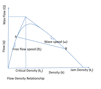
Density
Density (k) is defined as the number of vehicles per unit length of the roadway. In traffic flow, the two most important densities are the critical density (kc) and jam density (kj). The maximum density achievable under free flow is kc, while kj is the maximum density achieved under congestion. In general, jam density is seven times the critical density. Inverse of density is spacing (s), which is the center-to-center distance between two vehicles.

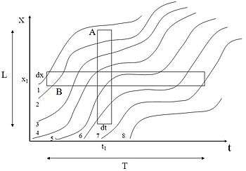
The density (k) within a length of roadway (L) at a given time (t1) is equal to the inverse of the average spacing of the n vehicles.

In a time-space diagram, the density may be evaluated in the region A.

where tt is the total travel time in A.
Flow
Flow (q) is the number of vehicles passing a reference point per unit of time, vehicles per hour. The inverse of flow is headway (h), which is the time that elapses between the ith vehicle passing a reference point in space and the (i + 1)th vehicle. In congestion, h remains constant. As a traffic jam forms, h approaches infinity.


The flow (q) passing a fixed point (x1) during an interval (T) is equal to the inverse of the average headway of the m vehicles.

In a time-space diagram, the flow may be evaluated in the region B.

where td is the total distance traveled in B.
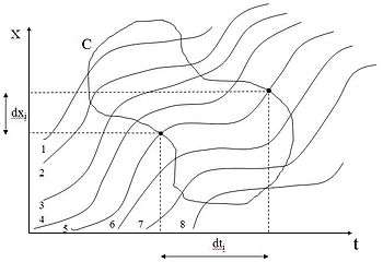
Generalized density and flow in time-space diagram
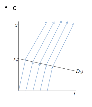
A more general definition of the flow and density in a time-space diagram is illustrated by region C:


where:


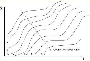
Congestion shockwave
In addition to providing information on the speed, flow, and density of traffic streams, time-space diagrams may illustrate the propagation of congestion upstream from a traffic bottleneck (shockwave). Congestion shockwaves will vary in propagation length, depending upon the upstream traffic flow and density. However, shockwaves will generally travel upstream at a rate of approximately 20 km/h.
Stationary traffic
Traffic on a stretch of road is said to be stationary if an observer does not detect movement in an arbitrary area of the time-space diagram. Traffic is stationary if all the vehicle trajectories are parallel and equidistant. It is also stationary if it is a superposition of families of trajectories with these properties (e.g. fast and slow drivers). By using a very small hole in the template one could sometimes view an empty region of the diagram and other times not, so that even in these cases, one could say that traffic was not stationary. Clearly, for such fine level of observation, stationary traffic does not exist. A microscopic level of observation must be excluded from the definition if traffic appears to be similar through larger windows. In fact, we relax the definition even further by only requiring that the quantities t(A) and d(A) be approximately the same, regardless of where the "large" window (A) is placed.
Methods of analysis
Analysts approach the problem in three main ways, corresponding to the three main scales of observation in physics:
- Microscopic scale: At the most basic level, every vehicle is considered as an individual. An equation can be written for each, usually an ordinary differential equation (ODE). Cellular automation models can also be used, where the road is divided into cells, each of which contains a moving car, or is empty. The Nagel–Schreckenberg model is a simple example of such a model. As the cars interact it can model collective phenomena such as traffic jams.
- Macroscopic scale: Similar to models of fluid dynamics, it is considered useful to employ a system of partial differential equations, which balance laws for some gross quantities of interest; e.g., the density of vehicles or their mean velocity.
- Mesoscopic (kinetic) scale: A third, intermediate possibility, is to define a function which expresses the probability of having a vehicle at time in position which runs with velocity . This function, following methods of statistical mechanics, can be computed using an integro-differential equation such as the Boltzmann equation.


The engineering approach to analysis of highway traffic flow problems is primarily based on empirical analysis (i.e., observation and mathematical curve fitting). One major reference used by American planners is the Highway Capacity Manual,[6] published by the Transportation Research Board, which is part of the United States National Academy of Sciences. This recommends modelling traffic flows using the whole travel time across a link using a delay/flow function, including the effects of queuing. This technique is used in many US traffic models and in the SATURN model in Europe.[7]
In many parts of Europe, a hybrid empirical approach to traffic design is used, combining macro-, micro-, and mesoscopic features. Rather than simulating a steady state of flow for a journey, transient "demand peaks" of congestion are simulated. These are modeled by using small "time slices" across the network throughout the working day or weekend. Typically, the origins and destinations for trips are first estimated and a traffic model is generated before being calibrated by comparing the mathematical model with observed counts of actual traffic flows, classified by type of vehicle. "Matrix estimation" is then applied to the model to achieve a better match to observed link counts before any changes, and the revised model is used to generate a more realistic traffic forecast for any proposed scheme. The model would be run several times (including a current baseline, an "average day" forecast based on a range of economic parameters and supported by sensitivity analysis) in order to understand the implications of temporary blockages or incidents around the network. From the models, it is possible to total the time taken for all drivers of different types of vehicle on the network and thus deduce average fuel consumption and emissions.
Much of UK, Scandinavian, and Dutch authority practice is to use the modelling program CONTRAM for large schemes, which has been developed over several decades under the auspices of the UK's Transport Research Laboratory, and more recently with the support of the Swedish Road Administration.[8] By modelling forecasts of the road network for several decades into the future, the economic benefits of changes to the road network can be calculated, using estimates for value of time and other parameters. The output of these models can then be fed into a cost-benefit analysis program.[9]
Cumulative vehicle count curves (N-curves)
A cumulative vehicle count curve, the N-curve, shows the cumulative number of vehicles that pass a certain location x by time t, measured from the passage of some reference vehicle.[10] This curve can be plotted if the arrival times are known for individual vehicles approaching a location x, and the departure times are also known as they leave location x. Obtaining these arrival and departure times could involve data collection: for example, one could set two point sensors at locations X1 and X2, and count the number of vehicles that pass this segment while also recording the time each vehicle arrives at X1 and departs from X2. The resulting plot is a pair of cumulative curves where the vertical axis (N) represents the cumulative number of vehicles that pass the two points: X1 and X2, and the horizontal axis (t) represents the elapsed time from X1 and X2.
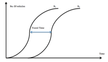
If vehicles experience no delay as they travel from X1 to X2, then the arrivals of vehicles at location X1 is represented by curve N1 and the arrivals of the vehicles at location X2 is represented by N2 in figure 8. More commonly, curve N1 is known as the arrival curve of vehicles at location X1 and curve N2 is known as the arrival curve of vehicles at location X2. Using a one-lane signalized approach to an intersection as an example, where X1 is the location of the stop bar at the approach and X2 is an arbitrary line on the receiving lane just across of the intersection, when the traffic signal is green, vehicles can travel through both points with no delay and the time it takes to travel that distance is equal to the free-flow travel time. Graphically, this is shown as the two separate curves in figure 8.
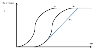
However, when the traffic signal is red, vehicles arrive at the stop bar (X1) and are delayed by the red light before crossing X2 some time after the signal turns green. As a result, a queue builds at the stop bar as more vehicles are arriving at the intersection while the traffic signal is still red. Therefore, for as long as vehicles arriving at the intersection are still hindered by the queue, the curve N2 no longer represents the vehicles’ arrival at location X2; it now represents the vehicles’ virtual arrival at location X2, or in other words, it represents the vehicles' arrival at X2 if they did not experience any delay. The vehicles' arrival at location X2, taking into account the delay from the traffic signal, is now represented by the curve N′2 in figure 9.
However, the concept of the virtual arrival curve is flawed. This curve does not correctly show the queue length resulting from the interruption in traffic (i.e. red signal). It assumes that all vehicles are still reaching the stop bar before being delayed by the red light. In other words, the virtual arrival curve portrays the stacking of vehicles vertically at the stop bar. When the traffic signal turns green, these vehicles are served in a first-in-first-out (FIFO) order. For a multi-lane approach, however, the service order is not necessarily FIFO. Nonetheless, the interpretation is still useful because of the concern with average total delay instead of total delays for individual vehicles.[11]
Step function vs. smooth function
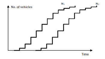
The traffic light example depicts N-curves as smooth functions. Theoretically, however, plotting N-curves from collected data should result in a step-function (figure 10). Each step represents the arrival or departure of one vehicle at that point in time.[11] When the N-curve is drawn on larger scale reflecting a period of time that covers several cycles, then the steps for individual vehicles can be ignored, and the curve will then look like a smooth function (figure 8).
N-curve: traffic flow characteristics
The N-curve can be used in a number of different traffic analyses, including freeway bottlenecks and dynamic traffic assignment. This is due to the fact that a number of traffic flow characteristics can be derived from the plot of cumulative vehicle count curves. Illustrated in figure 11 are the different traffic flow characteristics that can be derived from the N-curves.
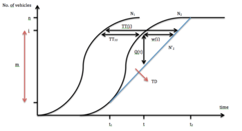
These are the different traffic flow characteristics from figure 11:
| Symbol | Definition |
|---|---|
| N1 | the cumulative number of vehicles arriving at location X1 |
| N2 | the virtual cumulative number of vehicles arriving at location X2, or the cumulative number of vehicles that would have liked to cross X2 by time t |
| N′2 | the actual cumulative number of vehicles arriving at location X2 |
| TTFF | the time it takes to travel from location X1 to location X2 at free-flow conditions |
| w(i) | the delay experienced by vehicle i as it travels from X1 to X2 |
| TT(i) | the total time it takes to travel from X1 to X2 including delays (TTFF + w(i)) |
| Q(t) | the queue at any time t, or the number of vehicles being delayed at time t |
| n | total number of vehicles in the system |
| m | total number of delayed vehicles |
| TD | total delay experienced by m vehicles (area between N2 and N′2) |
| t1 | time at which congestion begins |
| t2 | time at which congestion ends |
From these variables, the average delay experienced by each vehicle and the average queue length at any time t can be calculated, using the following formulas:


Hamilton Jacobi PDE
In traffic flow area, an alternative way to solve the kinematic wave model is to treat it like a Hamilton–Jacobi equation, which is particularly useful in identifying conserved quantities for mechanical systems.
Suppose we are interested in finding the cumulative curve as a function of time and space, N(t,x). Based the definition of cumulative curve, refers to the flow and refers to the density. Note that the sign convention should be consistent. Then the fundamental flow-density () equation: can be expressed in cumulative count form as:
, where is a known boundary.


Now, for a generic random point in the time-space diagram, the solution to the above partial derivative equation is equivalent to solve the following optimization problem, which minimizes the vehicles pass-by:, where is a random point on the boundary .


The function is defined as the maximum passing rate along the observers. In the case of triangular fundamental diagram, we have . The observer speed .Here, notation corresponds to the capacity, corresponds to the critical density, and are free flow speed and wave speed respectively.


With that being said, the minimization function above simplifies into: , where is a random point on the boundary . Here, we limit the solution discussion over initial value problems (IVP) and boundary value problems (BVP).

Initial value problem
Initial value problem occurs when boundary condition is given at a fixed time, e.g. at and boundary . As the observer speed is bounded by , the potential solution is delimited by two lines and .


Thus, the IVP is defined as follow:


The local minimum point occurs when the first order derivative is 0 and the second order derivative is greater than 0. Or, the minimum happens at boundaries. So, the set of potential solutions goes as follow:
1. that and
2. and .
The solution will be the minimum corresponding of all candidate points. and all from condition 1).


Specifically, if the initial condition is a linear function,


Boundary value problem
Similarly, the boundary value problem indicates the boundary condition is given at a fix location, e.g. . Still, the observer speed is bounded by . For a random point , the upper bound for solution candidates: if , ; else, .


The BVP is defined as follow:


The first order derivative: is always smaller than 0 because flows won't exceed the capacity. Thus, the minimum happens at the upper bound of the time axis.


In practice, people use this method to estimate the traffic states at between two loop detectors, which can be viewed as a combination of two boundary value problems (one at upstream and one at down stream). Denote the upstream loop detector location as and the downstream loop detector location as . Based on the conclusion above, the minimum value occurs at the upper bound along the time axis.
, with


Applications
The bottleneck model
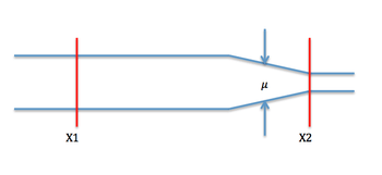
One application of the N-curve is the bottleneck model, where the cumulative vehicle count is known at a point before the bottleneck (i.e. this is location X1). However, the cumulative vehicle count is not known at a point after the bottleneck (i.e. this is location X2), but rather only the capacity of the bottleneck, or the discharge rate, μ, is known. The bottleneck model can be applied to real-world bottleneck situations such as those resulting from a roadway design problem or a traffic incident.
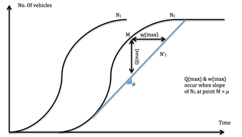
Take a roadway section where a bottleneck exists such as in figure 12. At some location X1 before the bottleneck, the arrivals of vehicles follow a regular N-curve. If the bottleneck is absent, the departure rate of vehicles at location X2 is essentially the same as the arrival rate at X1 at some later time (i.e. at time TTFF – free-flow travel time). However, due to the bottleneck, the system at location X2 is now only able to have a departure rate of μ. When graphing this scenario, essentially we have the same situation as in figure 9, where the arrival curve of vehicles is N1, the departure curve of vehicles absent the bottleneck is N2, and the limited departure curve of vehicles given the bottleneck is N′2. The discharge rate μ is the slope of curve N′2, and all the same traffic flow characteristics as in figure 11 can be determined from this diagram. The maximum delay and maximum queue length can be found at a point M in figure 13 where the slope of N2 is the same as the slope of N′2; i.e. when the virtual arrival rate is equal to the discharge / departure rate μ.
The N-curve in the bottleneck model may also be used to calculate the benefits in removing the bottleneck, whether in terms of a capacity improvement or removing an incident to the side of the roadway.
Tandem queues
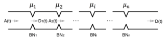
As introduced in the section above, the N-curve is an applicable model to estimate traffic delay during time by setting arrival and departure cumulative counting curve. Since the curve can represent various traffic characteristics and roadway conditions, the delay and queue situations under these conditions will be able to be recognized and modeled using N-curves. Tandem queues occur when multiple bottlenecks exist between the arrival and departure locations. Figure 14 shows a qualitative layout of a tandem-queue roadway segment with a certain initial arrival. The bottlenecks along the stream have their own capacity, 'μi [veh/time], and the departure is defined at the downstream end of the entire segment.
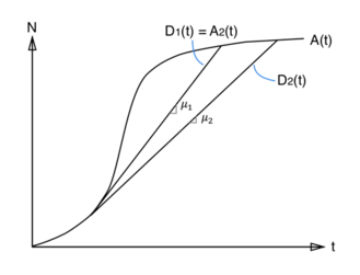
To determine the ultimate departure, D(t), it can be an available method to research on the individual departures, Di(t). As shown in the Figure 15, if the free-flow travel-time is neglected, the departure of BNi−1 will be the virtual arrival of BNi, which can also be presented as Di−1(t) = Ai(t). Thus, the N-curve of a roadway with two bottlenecks (minimum number of BNs along a tandem-queue roadway) can be developed as Figure 15 with μ1 < μ2. In this case, D2(t) will be the ultimate departure of this 2-BN tandem-queue roadway.
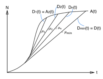
Regarding of a tandem-queue roadway having 3 BNs with μ1 < μ2, if μ1 < μ2 < μ3, similarly as the 2-BN case, D3(t) will be the ultimate departure of this 3-BN tandem-queue roadway. If, however, μ1 < μ3 < μ2, D2(t) will then still be the ultimate departure of the 3-BN tandem-queue roadway. Thus, it can be summarized that, the departure of the bottleneck with the minimum capacity will be the ultimate departure of the entire system, regardless of the other capacities and the number of bottlenecks. Figure 16 shows a general case with n BNs.
The N-curve model describing above represents a significant characteristic of the tandem-queue systems, which is that the ultimate departure only depends on the bottleneck with the minimum capacity. In a practical perspective, when the resources (economy, effort, etc.) of the investment on tandem-queue systems are limited, the investment can mainly focus on the bottleneck with the worst condition.
Traffic light

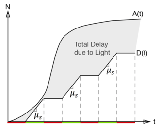
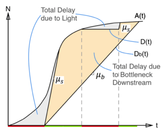
A signalized intersection will have special departure behaviors. With simplified speaking, a constant releasing free-flow capacity, μs, exists during the green phases. On the contrary, the releasing capacity during the red phases should be zero. Thus, the departure N-curve regardless of arrival will look like as Figure 17 below: counts increase with the slope of μs during green, and remain the same during red..
Saturated case of a traffic light occurs when the releasing capacity is fully used. This case usually exists when the arriving demand is relatively large. The N-curve representation of the saturated case is shown in the Figure 18.
Unsaturated case of a traffic light occurs when releasing capacity is not fully used. This case usually exists when the arriving demand is relatively small. The N-curve representation of the unsaturated case is shown in the Figure 19. If there is a bottleneck with a capacity of μb(<μs) downstream of the light, the ultimate departure of the light-bottleneck system will be that of the downstream bottleneck.
Dynamic traffic assignment
Dynamic traffic assignment can also be solved using the N-curve. There are two main approaches to tackle this problem: system optimum, and user equilibrium. This application will be discussed further in the following section.
Kerner’s three-phase traffic theory
Kerner’s three-phase traffic theory is an alternative theory of traffic flow. Probably the most important result of the three-phase theory is that at any time instance there is a range of highway capacities of free flow at a bottleneck. The capacity range is between some maximum and minimum capacities. The range of highway capacities of free flow at the bottleneck in three-phase traffic theory contradicts fundamentally classical traffic theories as well as methods for traffic management and traffic control which at any time instant assume the existence of a particular deterministic or stochastic highway capacity of free flow at the bottleneck.
Traffic assignment
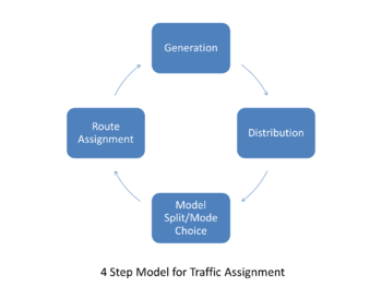
The aim of traffic flow analysis is to create and implement a model which would enable vehicles to reach their destination in the shortest possible time using the maximum roadway capacity. This is a four-step process:
- Generation – the program estimates how many trips would be generated. For this, the program needs the statistical data of residence areas by population, location of workplaces etc.;
- Distribution – after generation it makes the different Origin-Destination (OD) pairs between the location found in step 1;
- Modal Split/Mode Choice – the system has to decide how much percentage of the population would be split between the difference modes of available transport, e.g. cars, buses, rails, etc.;
- Route Assignment – finally, routes are assigned to the vehicles based on minimum criterion rules.
This cycle is repeated until the solution converges.
There are two main approaches to tackle this problem with the end objectives:
- System optimum
- User equilibrium
System optimum
In short, a network is in system optimum (SO) when the total system cost is the minimum among all possible assignments.
System Optimum is based on the assumption that routes of all vehicles would be controlled by the system, and that rerouting would be based on maximum utilization of resources and minimum total system cost. (Cost can be interpreted as travel time.) Hence, in a System Optimum routing algorithm, all routes between a given OD pair have the same marginal cost.
In traditional transportation economics, System Optimum is determined by equilibrium of demand function and marginal cost function. In this approach, marginal cost is roughly depicted as increasing function in traffic congestion. In traffic flow approach, the marginal cost of the trip can be expressed as sum of the cost(delay time, w) experienced by the driver and the externality(e) that a driver imposes on the rest of the users.[12]
Suppose there is a freeway(0) and an alternative route(1), which users can be diverted onto off-ramp. Operator knows total arrival rate(A(t)), the capacity of the freeway(μ_0), and the capacity of the alternative route(μ_1). From the time 't_0', when freeway is congested, some of the users start moving to alternative route. However, when 't_1', alternative route is also full of capacity. Now operator decides the number of vehicles(N), which use alternative route. The optimal number of vehicles(N) can be obtained by calculus of variation, to make marginal cost of each route equal. Thus, optimal condition is T_0=T_1+∆_1. In this graph, we can see that the queue on the alternative route should clear ∆_1 time units before it clears from the freeway. This solution does not define how we should allocates vehicles arriving between t_1 and T_1, we just can conclude that the optimal solution is not unique. If operator wants freeway not to be congested, operator can impose the congestion toll, e_0-e_1, which is the difference between the externality of freeway and alternative route. In this situation, freeway will maintain free flow speed, however alternative route will be extremely congested.
User equilibrium
In brief, A network is in user equilibrium (UE) when every driver chooses the routes in its lowest cost between origin and destination regardless whether total system cost is minimized.
The user optimum equilibrium assumes that all users choose their own route towards their destination based on the travel time that will be consumed in different route options. The users will choose the route which requires the least travel time. The user optimum model is often used in simulating the impact on traffic assignment by highway bottlenecks. When the congestion occurs on highway, it will extend the delay time in travelling through the highway and create a longer travel time. Under the user optimum assumption, the users would choose to wait until the travel time using a certain freeway is equal to the travel time using city streets, and hence equilibrium is reached. This equilibrium is called User Equilibrium, Wardrop Equilibrium or Nash Equilibrium.
The core principle of User Equilibrium is that all used routes between a given OD pair have the same travel time. An alternative route option is enabled to use when the actual travel time in the system has reached the free-flow travel time on that route.
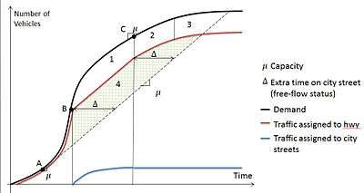
For a highway user optimum model considering one alternative route, a typical process of traffic assignment is shown in figure 15. When the traffic demand stays below the highway capacity, the delay time on highway stays zero. When the traffic demand exceeds the capacity, the queue of vehicle will appear on the highway and the delay time will increase. Some of users will turn to the city streets when the delay time reaches the difference between the free-flow travel time on highway and the free-flow travel time on city streets. It indicates that the users staying on the highway will spend as much travel time as the ones who turn to the city streets. At this stage, the travel time on both the highway and the alternative route stays the same. This situation may be ended when the demand falls below the road capacity, that is the travel time on highway begins to decrease and all the users will stay on the highway. The total of part area 1 and 3 represents the benefits by providing an alternative route. The total of area 4 and area 2 shows the total delay cost in the system, in which area 4 is the total delay occurs on the highway and area 2 is the extra delay by shifting traffic to city streets.
Navigation function in Google Maps can be referred as a typical industrial application of dynamic traffic assignment based on User Equilibrium since it provides every user the routing option in lowest cost (travel time).
Time delay
Both User Optimum and System Optimum can be subdivided into two categories on the basis of the approach of time delay taken for their solution:
Predictive Time Delay
Predictive time delay assumes that the user of the system knows exactly how long the delay is going to be right ahead. Predictive delay knows when a certain congestion level will be reached and when the delay of that system would be more than taking the other system, so the decision for reroute can be made in time. In the vehicle counts-time diagram, predictive delay at time t is horizontal line segment on the right side of time t, between the arrival and departure curve, shown in Figure 16. the corresponding y coordinate is the number nth vehicle that leaves the system at time t.
Reactive Time Delay
Reactive time delay is when the user has no knowledge of the traffic conditions ahead. The user waits to experience the point where the delay is observed and the decision to reroute is in reaction to that experience at the moment. Predictive delay gives significantly better results than the reactive delay method. In the vehicle counts-time diagram, predictive delay at time t is horizontal line segment on the left side of time t, between the arrival and departure curve, shown in Figure 16. the corresponding y coordinate is the number nth vehicle that enters the system at time t.

Kerner’s network breakdown minimization (BM) principle
Kerner introduced an alternative approach to traffic assignment based on his network breakdown minimization (BM) principle. Rather than an explicit minimization of travel time that is the objective of System Optimum and User Equilibrium, the BM principle minimizes the probability of the occurrence of congestion in a traffic network.[13] Under sufficient traffic demand, the application of the BM principle should lead to implicit minimization of travel time in the network.
Variable speed limit assignment
This is an upcoming approach of eliminating shockwave and increasing safety for the vehicles. The concept is based on the fact that the risk of accident on a roadway increases with speed differential between the upstream and downstream vehicles. The two types of crash risk which can be reduced from VSL implementation are the rear-end crash and the lane-change crash. Variable speed limits seek to homogenize speed, leading to a more constant flow.[14] Different approaches have been implemented by researchers to build a suitable VSL algorithm.
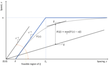
Variable speed limits are usually enacted when sensors along the roadway detect that congestion or weather events have exceeded thresholds. The roadway speed limit will then be reduced in 5-mph increments through the use of signs above the roadway (Dynamic Message Signs) controlled by the Department of Transportation. The goal of this process is the both increase safety through accident reduction and to avoid or postpone the onset of congestion on the roadway. The ideal resulting traffic flow is slower overall, but less stop-and-go, resulting in fewer instances of rear-end and lane-change crashes. The use of VSL’s also regularly employs shoulder-lanes permitted for transportation only under congested states which this process aims to combat. The need for a variable speed limit is shown by Flow-Density diagram to the right.
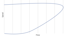
In this figure ("Flow-Speed Diagram for a Typical Roadway"), the point of the curve represents optimal traffic movement in both flow and speed. However, beyond this point the speed of travel quickly reaches a threshold and starts to decline rapidly. In order to reduce the potential risk of this rapid rate of speed decline, variable speed limits reduce the speed at a more gradual rate (5-mph increments), allowing drivers to have more time to prepare and acclimate to the slowdown due to congestion/weather. The development of a uniform travel speed reduces the probability of erratic driver behavior and therefore crashes.
Through historical data obtained at VSL sites, it has been determined that implementation of this practice reduces accident numbers by 20-30%.[14]
In addition to safety and efficiency concerns, VSL’s can also garner environmental benefits such as decreased emissions, noise, and fuel consumption. This is due to the fact that vehicles are more fuel-efficient when at a constant rate of travel, rather than in a state of constant acceleration and deacceleration like that usually found in congested conditions.[15]
Key Background Theory Fundamental relationships between volume (q), speed (u), and density (k) of traffic flow can explain the effectiveness of the VSL. The relationship between these variables is covered in the “Traffic stream properties” section of this page, but as an important takeaway for the purpose of VSL explanation, q=u*k. The Newell’s Simplified traffic flow theory is also utilized for this model to show the relationship displayed in the flow-density plot titled "Ideal Flow-Density Diagram".[16]
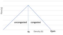
The figure "Ideal Flow-Density Diagram" shows there is a peak density that a roadway can sustain at an uncongested state, but if this density is surpassed then the roadway will fall into a congested traffic state. This density is known as the critical density, or KC. Shockwave theory is used in the VSL model to describe the effect of flow slow-down due to congestion. Shockwaves occur at the boundary between two different traffic flows, and their speeds can be shown as a ratio of a difference of density to the difference of volumes at the two traffic states.
A VSL often creates a void in the time-space diagram in the space between a vehicle’s trajectory at normal speed and a vehicle at the reduced speed within the VSL’s effective boundary. Below, the two forms of a variable speed limit are shown.
Initial Flow (“qA”) > Congested Upstream Flow (“qU”) (Case 1) When the initial roadway flow is greater than congested upstream flow, a shockwave is formed through the implementation of the VSL. The time-space diagram and flow-density fundamental diagram (simplified to a triangular diagram) are shown to the right. These diagrams represent a congested state. Please note that although the diagrams are not to scale with each other, the slopes representing the speed of the vehicle are equal in each state are the same in both diagrams.
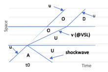
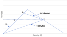
As apparent in the Case 1 diagrams, the introduction of a variable speed limit when initial flow is greater than congested upstream flow results in a void in the VSL zone (traffic state “O”). The VSL zone is shown by the horizontal lines. The normal free flow speed, u, is interrupted by the VSL resulting in a new speed of “v”. The introduction of the VSL introduces a shockwave as shown on both diagrams. The VSL implementation also introduces a new traffic state “U” for the VSL flowrate (instead of “A” at initial conditions) and a new traffic state “D” for downstream flows. Traffic states “D” and “U” share the same flow-rate but at different densities. The increase in speed back to “u” after the VSL zone leads to decreased density at state “D”. The shockwave caused by the VSL speed reduction begins to impact the roadway with traffic state “U” after a certain time of activity. This represents spillback of the controlled delay established by the VSL. The traffic state “U” has a higher density but the same flow as state “D”, which occurs after the VSL zone has passed.
Congested Upstream Flow “(qU”) > Initial Flow (“qA”) (Case 2) If congested upstream flow (denoted in the following diagrams by “U”) is greater than the initial roadway flow upstream (“A”), then the VSL will help to reduce the stop-and-go traffic, homogenizing traffic flow to result in traffic state “A” after its implementation. In the diagrams to the right for Case 2, assume all slopes are equal despite scale.


In the Case 2 diagrams, the implementation of VSL results in a reduced speed within the specified zone. However, as a result of the existing traffic states with qU>qA, traffic returns to initial state “A” after the VSL zone. A headway between vehicles “H” can be calculated between vehicle trajectories in the time-space diagram or at time qA/v on the flow-density fundamental diagram. In this form of the model, no alternate downstream traffic state is formed, and no shockwave due to congestion at the VSL occurs. The smaller triangle within the flow-density diagram represents the fundamental diagram for the VSL zone. In this zone, the traffic flow is normalized at a higher density but lower flow than the initial condition “A” due to the reduced speed of travel.
VSL Theory In showing the effectiveness of VSL, several key assumptions are made. 1. No entrance/exit ramps on freeway of analysis 2. Traffic flow analysis is based upon vehicle trajectory with no acceleration/deacceleration 3. Only passenger vehicles considered 4. Full compliance with VSL from all drivers 5. Focus on reducing congestion
Determining VSL Effectiveness VSL effectiveness can be verified quantitatively through analyzing the shockwaves formed by congestion with and without implementation. In the study cited throughout this section, shockwaves for an upstream incident were utilized for this comparison. One shockwave was formed through the congestion caused by an upstream incident, and the other was formed through this incident’s clearing and recovery to revert to normal flow. It was founded that the two shockwaves for a system with VSL implementation resulted in a much shorter delay and queue length due to the homogenization of flow through more rapid dissipation of the first shockwave. Through this study, the effectiveness of VSL in reducing congestion is proved, though with the limiting assumptions described above.
Limitations of VSL VSL implementation is most ideal under severe congestion states. If a reduced VSL is implemented in traffic states under critical density, then they will result in reduced flow overall through increased travel times. Thus, the benefits of VSL must be enacted carefully at only threshold states, which depend on the existing traffic data of the roadway. Therefore, sensors must be tuned effectively to detect when a congestive state will begin based upon historical data. The VSL must also begin before stop-and-go congested states of traffic are reached in order to be effective.
VSL effectiveness is also nearly completely based upon driver compliance. This can be ensured through enforcement and dynamic signage. Drivers must sense the legitimacy of the VSL for it to be effective; the reasoning for the new speed limit should be explained via signage in order to ensure compliancy. If the VSL is not viewed as mandatory by drivers, then it will not work effectively. If the VSL is reduced by a significant amount, compliance will reduce significantly. For this reason, most VSL speeds are above 40 mph on freeways. Several historical example show that compliance reduces at a much greater rate when the new speed limit falls below this threshold.
VSL systems are limited by the cost of the detectors and signage, which may exceed $5 million. The reduction of delay and accidents often offsets initial costs of implementation. It generally takes 1–2 years to effectively establish a VSL with driver compliance. 17
Road junctions
A major consideration in road capacity relates to the design of junctions. By allowing long "weaving sections" on gently curving roads at graded intersections, vehicles can often move across lanes without causing significant interference to the flow. However, this is expensive and takes up a large amount of land, so other patterns are often used, particularly in urban or very rural areas. Most large models use crude simulations for intersections, but computer simulations are available to model specific sets of traffic lights, roundabouts, and other scenarios where flow is interrupted or shared with other types of road users or pedestrians. A well-designed junction can enable significantly more traffic flow at a range of traffic densities during the day. By matching such a model to an "Intelligent Transport System", traffic can be sent in uninterrupted "packets" of vehicles at predetermined speeds through a series of phased traffic lights. The UK's TRL has developed junction modelling programs for small-scale local schemes that can take account of detailed geometry and sight lines; ARCADY for roundabouts, PICADY for priority intersections, and OSCADY and TRANSYT for signals. Many other junction analysis software packages[17] exist such as Sidra and LinSig and Synchro.
Kinematic wave model
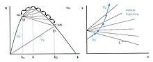
The kinematic wave model was first applied to traffic flow by Lighthill and Whitham in 1955. Their two-part paper first developed the theory of kinematic waves using the motion of water as an example. In the second half, they extended the theory to traffic on “crowded arterial roads.” This paper was primarily concerned with developing the idea of traffic “humps” (increases in flow) and their effects on speed, especially through bottlenecks.[18]
The authors began by discussing previous approaches to traffic flow theory. They note that at the time there had been some experimental work, but that “theoretical approaches to the subject [were] in their infancy.” One researcher in particular, John Glen Wardrop, was primarily concerned with statistical methods of examination, such as space mean speed, time mean speed, and “the effect of increase of flow on overtaking” and the resulting decrease in speed it would cause. Other previous research had focused on two separate models: one related traffic speed to traffic flow and another related speed to the headway between vehicles.[18]
The goal of Lighthill and Whitham, on the other hand, was to propose a new method of study “suggested by theories of the flow about supersonic projectiles and of flood movement in rivers.” The resulting model would capture both of the aforementioned relationships, speed-flow and speed-headway, into a single curve, which would “[sum] up all the properties of a stretch of road which are relevant to its ability to handle the flow of congested traffic.” The model they presented related traffic flow to concentration (now typically known as density). They wrote, “The fundamental hypothesis of the theory is that at any point of the road the flow q (vehicles per hour) is a function of the concentration k (vehicles per mile).” According to this model, traffic flow resembled the flow of water in that “Slight changes in flow are propagated back through the stream of vehicles along ‘kinematic waves,’ whose velocity relative to the road is the slope of the graph of flow against concentration.” The authors included an example of such a graph; this flow-versus-concentration (density) plot is still used today (see figure 3 above).[18]
The authors used this flow-concentration model to illustrate the concept of shock waves, which slow down vehicles which enter them, and the conditions that surround them. They also discussed bottlenecks and intersections, relating both to their new model. For each of these topics, flow-concentration and time-space diagrams were included. Finally, the authors noted that no agreed-upon definition for capacity existed, and argued that it should be defined as the “maximum flow of which the road is capable.” Lighthill and Whitham also recognized that their model had a significant limitation: it was only appropriate for use on long, crowded roadways, as the “continuous flow” approach only works with a large number of vehicles.[18]
Components of the kinematic wave model of traffic flow theory
The kinematic wave model of traffic flow theory is the simplest dynamic traffic flow model that reproduces the propagation of traffic waves. It is made up of three components: the fundamental diagram, the conservation equation, and initial conditions. The law of conservation is the fundamental law governing the kinematic wave model:

The fundamental diagram of the kinematic wave model relates traffic flow with density, as seen in figure 3 above. It can be written as:

Finally, initial conditions must be defined to solve a problem using the model. A boundary is defined to be , representing density as a function of time and position. These boundaries typically take two different forms, resulting in initial value problems (IVPs) and boundary value problems (BVPs). Initial value problems give the traffic density at time , such that , where is the given density function. Boundary value problems give some function that represents the density at the position, such that . The model has many uses in traffic flow. One of the primary uses is in modeling traffic bottlenecks, as described in the following section.


The Transport Equation
Assuming constant wave speed, , the kinematic wave model can be otherwise called the Transport equation, which is a key building block to a more simplified KW solution.

Initial Value Problem
Firstly, consider the initial value problem (IVP), that is, , for the transport equation:

k can thus be solved as . This is referred to as the IVP solution. This implies that along the lines with the same slope w on the space-time diagram, density k is constant. These lines are called characteristics. More specifically:


Boundary Value Problem
Consider the Boundary Value Problem (BVP), that is, , for the transport equation:


k can thus be solved as . This is referred to as the BVP solution. Similar to the IVP solution, this means that along the lines with the same slope w on the space-time diagram, or so called characteristics, density k remains constant.
It is assumed that when the initial conditions are piece wise constant, the wave speed of each piece is also constant thus the transport equation holds.
Riemann Problem
The Riemann problem provides the foundations to develop numeric solutions for the kinematic wave model. Consider the initial values:


Case 1:

This is a deceleration process, with traffic going from wave speed to , and density from to . The deceleration creates a discontinuity in traffic condition and results in a "shockwave":


The shockwave effect is illustrated in Figure 17. Traffic state moves from U (free flow) to D (congested). The slope s of this shockwave in the space time diagram is represented by the straight line that links point U and D.
Case 2:

This is an acceleration process, with traffic going from wave speed to , and density from to . The slope s of this shockwave can be same as to case 1, but that solution is not unique and the traffic state does not go back via a straight line from point D to U. Traffic recovers along the fundamental diagram curve, rather than returning to the free flow speed at once. This results in multiple different "solution shockwaves" that radiates from a given x0. These mechanism are shown in Figure 18.

In this case, oftentimes the entropy condition (EC) is used to pick a single solution. EC founds the solution that maximizes the flow at each location using the vanishing viscosity method.
Newell-Daganzo Merge Models
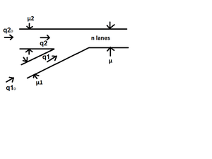
In the condition of traffic flows leaving two branch roadways and merging into a single flow through a single roadway, determining the flows that pass through the merging process and the state of each branch of roadways becomes an important task for traffic engineers. the Newell-Daganzo merge model is a good approach to solve these problems. This simple model is the output of the result of both Gordon Newell's description of the merging process[19] and the Daganzo's cell transmission model.[20] In order to apply the model to determine the flows which exiting two branch of roadways and the stat of each branch of roadways, one needs to know the capacities of the two input branches of roadways, the exiting capacity, the demands for each branch of roadways, and the number of lanes of the single roadway. The merge ratio will be calculated in order to determine the proportion of the two input flows when both of branches of roadway are operating in congested conditions.
As can be seen in a simplified model of the process of merging,[21] the exiting capacity of the system is defined to be μ, the capacities of the two input branches of roadways are defined as μ1 and μ2, and the demands for each branch of roadways are defined as q1D and q2D. The q1 and q2 are the output of the model which are the flows that pass through the merging process. The process of the model is based on the assumption that the sum of capacities of the two input branches of roadways is less than the exiting capacity of the system, μ1+μ2 ≤ μ.
Solution for Newell-Daganzo Merge Model
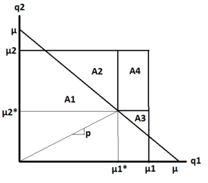
The flows that pass through the merging process, q1 and q2, are determined by split priority or, merge ratio. The state of each branch of roadways is determined by graphically with the input of the demands for each branch of roadways, q1D and q2D. There are four possible states for the merge system, both inlets in free flow, one of the inlets in congestion, and both inlets in congestion.
A common approach to calculate the merge ratio p is called "zipper rule" which p is calculated based on the number of lanes of the single roadway when both inlets are in congestion. If there are n lanes of the single roadway, then under the zipper rule, p=1/(2n-1). This merge ratio is also the ratio of minimum capacities of the inlets μ1* and μ2*. μ1* + μ2* = μ. As a result, q1=(μ1*/μ)*μ and q2=(μ2*/μ)*μ.
The state of each branch of roadways is determined by the graphical solution which is shown in the right. The x-axis is the possible value of q1 and the y-axis is the possible value of q2.The feasible region of demands is the defined by the maximum possible values for q1D and q2D which are μ1 and μ2. The feasible region for q1 and q2 is defined as the intersection between the line of q1 + q2 = μ and the feasible region of demands. The merge ration, p, is plotted from the origin to the line of q1 + q2 = μ.
The four possible states of the merge system are shown in the graph by the regions noted by A1, A2, A3, and A4. A specific states of a merge system is determined by the region where the input data fall into. The region A1 represents the state when both inlet 1 and inlet 2 are in free flow. The region A2 represents the state when inlet 1 is in free flow and inlet 2 is in congestion. The region A3 represents the state when inlet 1 is in congestion and inlet 2 is in free flow. The region A4 represents the state when both inlet 1 and inlet 2 are in congestion.
Traffic bottleneck
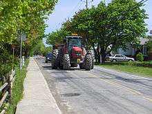
Traffic bottlenecks are disruptions of traffic on a roadway caused either due to road design, traffic lights, or accidents. There are two general types of bottlenecks, stationary and moving bottlenecks. Stationary bottlenecks are those that arise due to a disturbance that occurs due to a stationary situation like narrowing of a roadway, an accident. Moving bottlenecks on the other hand are those vehicles or vehicle behavior that causes the disruption in the vehicles which are upstream of the vehicle. Generally, moving bottlenecks are caused by heavy trucks as they are slow moving vehicles with less acceleration and also may make lane changes.

Bottlenecks are important considerations because they impact the flow in traffic, the average speeds of the vehicles. The main consequence of a bottleneck is an immediate reduction in capacity of the roadway. The Federal Highway Authority has stated that 40% of all congestion is from bottlenecks figure 16 shows the pie-chart for various causes of congestion. Figure 17[22] shows the common causes of congestion or bottlenecks.
Stationary bottleneck
The general cause of stationary bottlenecks are lane drops which occurs when the a multilane roadway loses one or more its lane. This causes the vehicular traffic in the ending lanes to merge onto the other lanes.
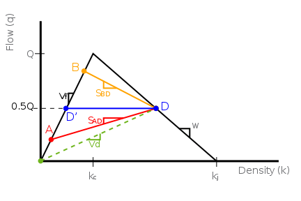
Consider a stretch of highway with two lanes in one direction. Suppose that the fundamental diagram is modeled as shown here. The highway has a peak capacity of Q vehicles per hour, corresponding to a density of kc vehicles per mile. The highway normally becomes jammed at kj vehicles per mile.
Before capacity is reached, traffic may flow at A vehicles per hour, or a higher B vehicles per hour. In either case, the speed of vehicles is vf, or "free flow," because the roadway is under capacity.
Now, suppose that at a certain location x0, the highway narrows to one lane. The maximum capacity is now limited to D', or half of Q, since only one lane of the two is available. D shares the same flowrate as state D', but its vehicular density is higher.

Using a time-space diagram, we may model the bottleneck event. Suppose that at time 0, traffic begins to flow at rate B and speed vf. After time t1, vehicles arrive at the lower flowrate A.
Before the first vehicles reach location x0, the traffic flow is unimpeded. However, downstream of x0, the roadway narrows, reducing the capacity by half – and to below that of state B. Due to this, vehicles will begin queuing upstream of x0. This is represented by high-density state D. The vehicle speed in this state is the slower vd, as taken from the fundamental diagram. Downstream of the bottleneck, vehicles transition to state D', where they again travel at free-flow speed vf.
Once vehicles arrive at rate A starting at t1, the queue will begin to clear and eventually dissipate. State A has a flowrate below the one-lane capacity of states D and D'.
On the time-space diagram, a sample vehicle trajectory is represented with a dotted arrow line. The diagram can readily represent vehicular delay and queue length. It is a simple matter of taking horizontal and vertical measurements within the region of state D.
Moving bottleneck
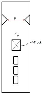
As explained above, moving bottlenecks are caused due to slow moving vehicles that cause disruption in traffic. Moving bottlenecks can be active or inactive bottlenecks. If the reduced capacity(qu) caused due to a moving bottleneck is greater than the actual capacity(μ) downstream of the vehicle, then this bottleneck is said to be an active bottleneck. Figure 20 shows the case of a truck moving with velocity 'v' approaching a downstream location with capacity 'μ'. If the reduced capacity of the truck (qu) is less than the downstream capacity, then the truck becomes an inactive bottleneck.
Laval 2009, presents a framework for estimating analytical expressions for the capacity reductions caused by a subset of vehicles forced to slow down at horizontal/vertical curves on multilane freeway. In each of the lane the underperforming stream is described in terms of its desired speed distribution and is modeled as per Newell’s kinematic wave theory for moving bottlenecks. Lane changing in the presence of trucks can lead to a positive or negative impact on capacity. If the target lane is empty then the lane-changing increases capacity
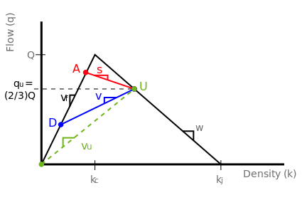
For this example, consider three lanes of traffic in one direction. Assume that a truck starts traveling at speed v, slower than the free flow speed vf. As shown on the fundamental diagram below, qu represents the reduced capacity (2/3 of Q, or 2 of 3 lanes available) around the truck.
State A represents normal approaching traffic flow, again at speed vf. State U, with flowrate qu, corresponds to the queuing upstream of the truck. On the fundamental diagram, vehicle speed vu is slower than vf. But once drivers have navigated around the truck, they can again speed up and transition to downstream state D. While this state travels at free flow, the vehicle density is less because fewer vehicles get around the bottleneck.
Suppose that, at time t, the truck slows from free-flow to v. A queue builds behind the truck, represented by state U. Within the region of state U, vehicles drive slower as indicated by the sample trajectory. Because state U limits to a smaller flow than state A, the queue will back up behind the truck and eventually crowd out the entire highway (slope s is negative). If state U had the higher flow, there would still be a growing queue. However, it would not back up because the slope s would be positive.

Riemann's problem
Imagine a scenario in which a two lane road is reduced to one lane at point xo from here on the road’s capacity is reduced to half its original (½µ), Case I. Later along the road at point x1 the 2nd lane is opened and the capacity is restored to its original (µ), Case II.
- Case I
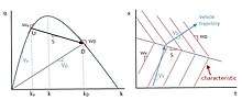
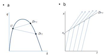
There is a bottleneck limiting the flow of traffic which causes an increase in the density of cars (k) at location (xo). This causes a deceleration for all oncoming cars traveling at speed u to slow to speed vd. This shockwave will travel at the speed of the slope of line U-D on the fundamental diagram. The wave speed can be calculated as vshock = (qD − qU)/(kD−kU). This line delineates the congestion traffic from oncoming free-flow traffic. If the slope of U-D on the fundamental diagram is positive congestion will continue downstream of the highway. If it has a negative slope the congestion will continue upstream (see figure a[22]). This deceleration is the case I of Riemann’s problem (see figure b and c).
- Case II
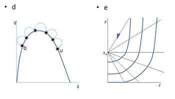
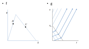
In case II of Riemann’s problem traffic goes from congestion to free-flow and the cars accelerate as the density drops. Again the slope of these shock waves can be calculated using the same formula vshock = (qD − qU)/(kD−kU). The difference this time is that traffic flow travels along the fundamental diagram not in a straight line across but many slopes between various points on the curved fundamental diagram (see figure d). This causes many lines emanating from point x1 all in a fan shape, called rarefaction (see figure e). This model implies that the users later on in time will take longer to accelerate as they meet each of the lines. Instead a better approximation is a triangular diagram where the traffic increases abruptly as it would when a driver sees an opening in front of them (see figures f and g).
Criticism
In a critical review,[23] Kerner explained that generally accepted classical fundamentals and methodologies of traffic and transportation theory are inconsistent with the set of fundamental empirical features of traffic breakdown at a highway bottleneck.
Set of fundamental empirical features of traffic breakdown at highway bottlenecks
The set of fundamental empirical features of traffic breakdown at a highway bottleneck is as follows:
- Traffic breakdown at a highway bottleneck is a local phase transition from free flow (F) to congested traffic whose downstream front is usually fixed at the bottleneck location. Such congested traffic is called synchronized flow (S). Within the downstream front of synchronized flow, vehicles accelerate from synchronized flow upstream of the bottleneck to free flow downstream of the bottleneck.
- At the same bottleneck, traffic breakdown can be either spontaneous or induced.
- The probability of traffic breakdown is an increasing flow rate function.
- There is a well-known hysteresis phenomenon associated with traffic breakdown: When the breakdown has occurred at some flow rates with resulting congested pattern formation upstream of the bottleneck, then a return transition to free flow at the bottleneck is usually observed at considerably smaller flow rates.
A spontaneous traffic breakdown occurs, where there are free flows both upstream and downstream of the bottleneck before the breakdown has occurred. In contrast, an induced traffic breakdown is caused by a propagation of a congested pattern that has earlier emerged for example at another downstream bottleneck.
Empirical data that illustrates the set of fundamental empirical features of traffic breakdown at highway bottlenecks as well as explanations of the empirical data can be found in Wikipedia article Kerner’s breakdown minimization principle and in review.[23]
Classical traffic flow theories
The generally accepted classical fundamentals and methodologies of traffic and transportation theory are as follows:
(i) The Lighthill-Whitham-Richards (LWR) model introduced in 1955–56.[18][24] Daganzo introduced a cell-transmission model (CTM) that is consistent with the LWR model.[25]
(ii) A traffic flow instability that causes a growing wave of a local reduction of the vehicle speed. This classical traffic flow instability was introduced in 1959–61 in the General Motors (GM) car-following model by Herman, Gazis, Montroll, Potts, and Rothery.[26][27] The classical traffic flow instability of the GM model has been incorporated in a huge number of traffic flow models like Gipps's model, Payne's model, Newell's optimal velocity (OV) model, Wiedemann's model, Whitham's model, the Nagel-Schreckenberg (NaSch) cellular automaton (CA) model, Bando et al. OV model, Treiber's IDM, Krauß model, the Aw-Rascle model and many other well-known microscopic and macroscopic traffic-flow models, which are the basis of traffic simulation tools widely used by traffic engineers and researchers (see, e.g., references in review[23]).
(iii) The understanding of highway capacity as a particular value. This understanding of road capacity was probably introduced in 1920–35 (see [28]). Currently, it is assumed that highway capacity of free flow at a highway bottleneck is a stochastic value. However, in accordance with the classical understanding of highway capacity, it is assumed that at a given time instant there can be only one particular value of this stochastic highway capacity (see references in the book[29]).
(iv) Wardrop's user equilibrium (UE) and system optimum (SO) principles for traffic and transportation network optimization and control.[30] –
Failure of classical traffic flow theories
Kerner explains the failure of the generally accepted classical traffic flow theories as follows:[23]
1. The LWR-theory fails because this theory cannot show empirical induced traffic breakdown observed in real traffic. Correspondingly, all applications of LWR-theory to the description of traffic breakdown at highway bottlenecks (like related applications of Daganzo’s cell-transmission model, cumulative vehicle count curves (N-curves), bottleneck model, highway capacity models as well as associated applications of kinematic wave theory) are also inconsistent with the set of fundamental empirical features of traffic breakdown.
2. Two-phase traffic flow models of the GM model class (see references in[23]) fail because traffic breakdown in the models of the GM class is a phase transition from free flow (F) to a moving jam (J) (called F → J transition): In a traffic flow model belonging to the GM model class due to traffic breakdown, a moving jam(s) appears spontaneously in an initially free flow at a highway bottleneck. In contrast with this model result, real traffic breakdown is a phase transition from free flow (F) to synchronized flow (S) (called F → S transition): Rather than a moving jam(s), due to traffic breakdown in real traffic, synchronized flow occurs whose downstream front is fixed at the bottleneck.
3. The understanding of highway capacity as a particular value (see references in the book [29]) fails because this assumption about the nature of highway capacity contradicts the empirical evidence that traffic breakdown can be induced at a highway bottleneck.
4. Dynamic traffic assignment or/and any kind of traffic optimization and control based on Wardrop's SO or UE principles fail because of possible random transitions between the free flow and synchronized flow at highway bottlenecks. Due to such random transitions, the minimization of travel cost in a traffic network is not possible.
According to Kerner,[23] the inconsistence the generally accepted classical fundamentals and methodologies of traffic and transportation theory with the set of fundamental empirical features of traffic breakdown at a highway bottleneck can explain why network optimization and control approaches based on these fundamentals and methodologies have failed by their applications in the real world. Even several decades of a very intensive effort to improve and validate network optimization models have no success. Indeed, there can be found no examples where on-line implementations of the network optimization models based on these fundamentals and methodologies could reduce congestion in real traffic and transportation networks.
This is due to the fact that the fundamental empirical features of traffic breakdown at highway bottlenecks have been understood only during last 20 years. In contrast, the generally accepted fundamentals and methodologies of traffic and transportation theory have been introduced in the 50s-60s. Thus the scientists whose ideas led to these classical fundamentals and methodologies of traffic and transportation theory could not know the set of empirical features of real traffic breakdown.
Incommensurability of Kerner’s three-phase traffic theory and classical traffic-flow theories
The explanation of traffic breakdown at a highway bottleneck by a F → S transition in a metastable free flow at the bottleneck is the basic assumption of Kerner’s three-phase traffic theory.[23] The three-phase traffic theory is consistent with the set of fundamental empirical features of traffic breakdown. None of earlier traffic-flow theories incorporates a F→S transition in a metastable free flow at the bottleneck. Therefore, as above mentioned none of the classical traffic flow theories is consistent with the set of empirical features of real traffic breakdown at a highway bottleneck. The F→S phase transition in metastable free flow at highway bottleneck does explain the empirical evidence of the induced transition from free flow to synchronized flow together with the flow-rate dependence of the breakdown probability. In accordance with the classical book by Kuhn,[31] this shows the incommensurability of three-phase theory and the classical traffic-flow theories (for more details, see [32]):
The minimum highway capacity , at which the F→S phase transition can still be induced at a highway bottleneck as stated in Kerner’s theory, has no sense for other traffic flow theories and models.

The term "incommensurability" has been introduced by Kuhn in his classical book[31] to explain a paradigm shift in a scientific field. The existence of these two traffic phases, free flow (F) and synchronized flow (S) at the same flow rate does not result from the stochastic nature of traffic: Even if there were no stochastic processes in vehicular traffic, the states F and S do exist at the same flow rate. However, classical stochastic approaches to traffic control do not assume a possibility of an F→S phase transition in metastable free flow. For this reason, these stochastic approaches cannot resolve the problem of the inconsistence of classical theories with the set of empirical features of real traffic breakdown.
Car-following models
Car-following models describe how one vehicle follows another vehicle in an uninterrupted traffic flow.
Introduction to three representations of traffic flow
There're three representations of traffic flow, all these three representations are corresponding to the same surface in the three-dimensional space of vehicle number, position, and time:
- N(t,x): the number of vehicles that have crossed location x by the time t, represented in Eulerian coordinates (t,x).
- X(t,n): the position of vehicle n at the time t, represented in Lagrangian coordinates (t,n).
- T(n,x): the time of vehicle n crosses position x, represented in Lagrangian coordinates (n,x).
Based on the theory of Hamilton-Jacobi equation aforementioned, the solutions (Hopf-Lax formula) of the three models can be represented as:


For the N(t,x) model, the Hamilton-Jacobi PDE is based on the density-flow fundamental diagram, the Lagrangian function can be represented as , in the case of trangle fundamental diagram, , is the wave speed, is the critical density, is the capacity. For the X(t,n) model, the Hamilton-Jacobi PDE is based on the spacing-speed fundamental diagram, the Lagrangian function can be represented as , in the case of trangle fundamental diagram, , is the wave flow, is the critical spacing, is the free flow speed. For the T(n,x) model, the Hamilton-Jacobi PDE is based on the pace-headway fundamental diagram, the Lagrangian function can be represented as , in the case of trangle fundamental diagram, , is the wave spacing, is the free flow speed, is the capacity.


Note that of each model is described in the table below:

| Initial Value Problem | Boundary Value Problem | |
|---|---|---|
| : cumulative vehicle profile at | : cumulative cout curve at | |
| : position of vehicle n at | : trajectory of leading vehicle | |
| : trajectory of leading vehicle | : time for vehicle n enter the road segment |


X-models
.png)
Considering the triangular flow-density fundamental diagram, we can get and , and correspondingly the car-following model can be described via model:


where is the headway between vehicles, and the bumper-to-bumper spacing at which vehicles are jamed can be derived as . The solution of can be graphically shown in Figure 28 and Figure 29.

When the constant spacing is applied, the initial data is linear, and the car-following model can be simplified into:

Then, if we partition the time-space plane into grids of , and we interpret the origin (0,0) as , the general car-following model becomes:


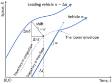
The solution can be interpreted intuitively in the time-space diagram of Figure 30: the trajectory vehicle n is the lower envelope between (i) the trajectory of leading vehicle shifting along the characteristics of slope , and (ii) its own trajectory under free-flow conditions.

However, the general car-following model assumes an infinite vehicle acceleration, which is impractical. To compensate for this drawback, we can incorporate a vehicle kinematics model into the car-following model. The vehicle kinematics can be expressed as a linear acceleration model:

in which is the acceleration coefficient, is the desirable speed.
Define as the resulting displacement at time for vehicle starting at a speed of at time 0, the general-car following model with acceleration bounds would be:


Examples of car-following models
Newell's car-following model
Recall the general car-following model we obtain from X-model above, Newell's car-following model can be derived via setting and :


in which represents vehicle trajectory in the free-flow conditions, and is the vehicle trajectory in congested conditions.


Some additional explanations and examples can be found in Wikipedia webpage Newell's car-following model.
Pipes model
Louis A. Pipes started researching and gaining acknowledgment from the public in the early 1950s. Pipes car-following model [33] is based on a safe driving rule in the California Motor Vehicle Code, and this model utilized an assumption of safe distance: a good rule for following another vehicle is to allocate an inter-vehicle distance of at least the length of a car for every ten miles per hour of vehicle speed. Mathematically, the safety spacing in Pipes car-following model can be derived as:

in which is the inter-vehicle distance between vehicle and preceding vehicle , and is the absolute position of vehicle and vehicle respectively, is the speed of vehicle , and is the length of vehicle and vehicle respectively, is the coefficient of unit conversion from mph to m/s.


More specifically, the safe spacing and safe time headway in Pipes car-following model can be expressed as:


Newell nonlinear model
To capture the potential nonlinear effects in the dynamics of car following, G. F. Newell proposed a nonlinear car-following model[34] based on empirical data. Unlike Pipes model which is solely relying on rules of safe driving, Newell nonlinear model aims at capturing the correct shape of fundamental diagrams (e.g., density-speed, flow-speed, density-flow, spacing-speed, pace-headway, etc.). The Newell nonlinear model can be described as:

in which is the speed of vehicle , is the perception-reaction time of driver , is the desirable speed, is the parameter associated with driver , is the spacing between vehicle and preceding vehicle , is the length of vehicle .


Optimal velocity model
The Optimal Velocity Model (OVM) is introduced by Bando et al. in 1995 [35] based on the assumption that each driver tries to reach to the optimal velocity according to the inter-vehicle difference and velocity difference between preceding vehicle. In OVM, the acceleration/deceleration of vehicle n is a function of inter-vehicle distance , speed of preceding vehicle , and sensitivity coefficient (which represents driver's sensitivity towards acceleration, large value indicates an aggressive driver while small value means a cautious driver):


in which is the Optimal Velocity function (OV-function), it can be expressed as:


The OV-function has two following properties:
1. The OV-function is a monotone increasing function.
2. has an upper-bound:


Intelligent driver model
Intelligent driver model is widely adopted in the research of Connected Vehicle (CV) and Connected and Autonomous Vehicle (CAV). For details about this car-following model, see Wikipedia webpage Intelligent driver model.
See also
- Braess's paradox
- Data flow
- Dijkstra's algorithm
- Epidemiology of motor vehicle collisions
- Floating car data
- Infrared traffic logger
- Truck lane restriction
- Road traffic control
- Road traffic safety#Statistics
- Rule 184
- Traffic counter
- Traffic engineering
- Turning movement counters
References
- Henry Lieu (January–February 1999). "Traffic-Flow Theory". Public Roads (Vol. 62· No. 4).
- Rijn, John. "Road Capacities" (PDF). Indevelopment. Retrieved 22 July 2014.
- V.L. Knoop and W. Daamen (2017). "Automatic fitting procedure for the fundamental diagram". Transportmetrica B: Transport Dynamics. 5 (2): 133–148. doi:10.1080/21680566.2016.1256239.
- Laval, Jorge A.; Toth, Christopher S.; Zhou, Yi (2014-12-01). "A parsimonious model for the formation of oscillations in car-following models". Transportation Research Part B: Methodological. 70: 228–238. doi:10.1016/j.trb.2014.09.004. ISSN 0191-2615.
- Lint, J. W. C. V., "Reliable travel time prediction for freeways", Phd thesis, Netherlands TRAIL Research School, 2004
- Highway Capacity Manual 2000
- SATURN ITS Transport Software Site
- Introduction to Contram
- UK Department for Transport's WebTag guidance on the conduct of transport studies
- Cassidy, M.J.; Bertini, R.L. (1999). "Some Traffic Features at Freeway Bottlenecks". Transportation Research Part B: Methodological. 33 (1): 25–42. doi:10.1016/S0191-2615(98)00023-X.
- Pitstick, Mark E. "Measuring Delay and Simulating Performance at Isolated Signalized Intersections Using Cumulative Curves." Transportation Research Record 1287 (1990)
- Juan Carlos Muñoz and Jorge A. Laval. “System optimum dynamic traffic assignment graphical solution method for a congested freeway and one destination”. Transportation Research Part B : Methodological (2006)
- Minimizing the probability of the occurrence of traffic congestion in a traffic network
- Xu, Wang (2016). "Implementation of Variable Speed Limits: Preliminary Test on Whitemud Drive, Edmonton, Canada". Journal of Transportation Engineering. 142 (12): 05016007. doi:10.1061/(ASCE)TE.1943-5436.0000895.
- Texas A&M Transportation Institute. "Variable Speed Limits" (PDF). Traffic Management. Texas A&M. Retrieved 2018-12-03.
- Laval, Jorge (2018). Traffic Flow Theory.
- Mahmud, Khizir; Town, Graham E. (June 2016). "A review of computer tools for modeling electric vehicle energy requirements and their impact on power distribution networks". Applied Energy. 172: 337–359. doi:10.1016/j.apenergy.2016.03.100.
- Lighthill, M.J.; Whitham, G.B. (1955). "On kinematic waves. I: Flood movement in long rivers. II: A theory of traffic flow on long crowded roads". Proceedings of the Royal Society. 229A (4): 281–345.
- Newell, Gordon (1982). Applications of Queueing Theory (2nd ed.). London: Chapman and Hall.
- Daganzo, Carlos (1994). "The Cell Transmission Model, part II: Network Traffic". Transportation Research Part B: Methodological. 28 (2): 279–293.
- Cassidy, Michael J.; Ahn, Soyoung (2005). "Driver Turn-Taking Behavior in Congested Freeway Merges" (PDF). Transportation Research Record: Journal of the Transportation Research Board. 1934: 140–147. CiteSeerX 10.1.1.367.2080. doi:10.3141/1934-15.
- figure missing
- Kerner, Boris S. (2013). "Criticism of generally accepted fundamentals and methodologies of traffic and transportation theory: A brief review". Physica A: Statistical Mechanics and Its Applications. 392 (21): 5261–5282. Bibcode:2013PhyA..392.5261K. doi:10.1016/j.physa.2013.06.004.
- P.I. Richards, "Shockwaves on the highway". Oper. Res., 4, 42-51 (1956)
- Daganzo, Carlos F. (1994). "The cell transmission model: A dynamic representation of highway traffic consistent with the hydrodynamic theory". Transportation Research Part B: Methodological. 28 (4): 269–287. doi:10.1016/0191-2615(94)90002-7.
- R. Herman, E.W. Montroll, R.B. Potts, and R.W. Rothery, "Traffic dynamics: analysis of stability in car following". Oper. Res. , 7, 86-106 (1959)
- D.C. Gazis, R. Herman, and R.W. Rothery. "Nonlinear follow-the-leader models of traffic flow". Oper. Res., 9, 545-567 (1961)
- Greenshields, B.D. "A study of traffic capacity". Highway Research Board Proceedings, 14, 448–477 (1935) )
- Elefteriadou, L. "An Introduction to Traffic Flow Theory". Springer Optimization and Its Applications, Vol. 84 (Springer, Berlin 2014)
- J.G. Wardrop, "Some theoretical aspects of road traffic research", in Proc. of Inst. of Civil Eng. II., 1, 325—362 (1952)
- T.S. Kuhn, "The structure of scientific revolutions". Fourth edition. (The University of Chicago Press, Chicago, London 2012)
- Kerner, Boris S.; Klenov, Sergey L.; Schreckenberg, Michael (2014). "Probabilistic physical characteristics of phase transitions at highway bottlenecks: Incommensurability of three-phase and two-phase traffic-flow theories". Phys. Rev. E. 89 (5): 052807. Bibcode:2014PhRvE..89e2807K. doi:10.1103/PhysRevE.89.052807. PMID 25353844.
- Pipes, Louis A. (1953). "An Operational Analysis of Traffic Dynamics". Journal of Applied Physics. 24 (3): 274–281. Bibcode:1953JAP....24..274P. doi:10.1063/1.1721265.
- Newell, G. F. (1961). "Nonlinear Effects in the Dynamics of Car Following". Operations Research. 9 (2): 209–229. doi:10.1287/opre.9.2.209. JSTOR 167493.
- Bando, M.; Hasebe, K.; Nakayama, A.; Shibata, A.; Sugiyama, Y. (1995). "Dynamical model of traffic congestion and numerical simulation". Physical Review E. 51 (2): 1035–1042. Bibcode:1995PhRvE..51.1035B. doi:10.1103/PhysRevE.51.1035. PMID 9962746.
Further reading
A survey about the state of art in traffic flow modeling:
- N. Bellomo, V. Coscia, M. Delitala, On the Mathematical Theory of Vehicular Traffic Flow I. Fluid Dynamic and Kinetic Modelling, Math. Mod. Meth. App. Sc., Vol. 12, No. 12 (2002) 1801–1843
- S. Maerivoet, Modelling Traffic on Motorways: State-of-the-Art, Numerical Data Analysis, and Dynamic Traffic Assignment, Katholieke Universiteit Leuven, 2006
- M. Garavello and B. Piccoli, Traffic Flow on Networks, American Institute of Mathematical Sciences (AIMS), Springfield, MO, 2006. pp. xvi+243 ISBN 978-1-60133-000-0
- Carlos F.Daganzo, "Fundamentals of Transportation and Traffic Operations.", Pergamon-Elsevier, Oxford, U.K. (1997)
- B.S. Kerner, Introduction to Modern Traffic Flow Theory and Control: The Long Road to Three-Phase Traffic Theory, Springer, Berlin, New York 2009
- Cassidy, M.J. and R.L. Bertini. "Observations at a Freeway Bottleneck." Transportation and Traffic Theory (1999).
- Daganzo, Carlos F. "A Simple Traffic Analysis Procedure." Networks and Spatial Economics 1.i (2001): 77–101.
- Lindgren, Roger V.F. "Analysis of Flow Features in Queued Traffic on a German Freeway." Portland State University (2005).
- Ni, B. and J.D. Leonard. "Direct Methods of Determining Traffic Stream Characteristics by Definition." Transportation Research Record (2006).
Useful books from the physical point of view:
- M. Treiber and A. Kesting, "Traffic Flow Dynamics", Springer, 2013
- B.S. Kerner, The Physics of Traffic, Springer, Berlin, New York 2004
- Traffic flow on arxiv.org
- May, Adolf. Traffic Flow Fundamentals. Prentice Hall, Englewood Cliffs, NJ, 1990.
- Taylor, Nicholas. The Contram dynamic traffic assignment model TRL 2003