Time–distance diagram
A time–distance diagram is generally a diagram with one axis representing time and the other axis distance. Such charts are used in the aviation industry to plot flights,[1] or in scientific research to present effects in respect to distance over time. Transport schedules in graphical form are also called time–distance diagrams,[2] they represent the location of a given vehicle (train, bus) along the transport route.[3]

In project management, a time–distance diagram (other names: Time-chainage diagram, Time–distance chart, Time-chainage chart, Time–location diagram, Time-location chart, March chart, Location–time chart, Orthogonal Diagram, Line of balance chart,[4] Linear Schedule or Horse Blanket Diagram[5]), is a method of graphically presenting a time schedule for all types of longitudinal projects such as pipeline, rail, bridge, tunnel, road, and transmission line construction. Activities in time–distance diagrams are displayed both along a time axis and along a distance axis according to their relative linear position. This allows showing not only the location of the activity but also the direction of progress and the progress rate. Activities can be presented as geometrical shapes showing the occupation of the work site over time such that conflicting access can be detected visually. Different types of activities are differentiated by color, fill pattern, line type, or special symbols. A symbolic drawing along the distance axis is often used to improve the understanding of the time–distance diagram.
The advantage of a time–distance diagram is that it nicely shows all visible activities along the construction site on a single diagram.
Layout
A time–distance diagram is a chart with two axes: one for time, the other for location. The units on either axis depend on the type of project: time can be expressed in minutes (for overnight construction of railroad modification projects such as the installation of switches) or years (for large construction projects); the location can be (kilo)meters, or other distinct units (such as stories of a high-rise building).
Normally, the time axis is drawn vertically from top (start of project) to bottom (end of project), and the location axis is drawn horizontally. The direction of the chainage is usually chosen with consideration of geographical position of the project, with the numbers either increasing or decreasing. The location axis is often enhanced with a schematic of the construction project. Other, location-specific information (aerial photos, cross-sectional views) can be added to enhance the visualization of the work site.
A legend explaining the meaning of the various colors, symbols and line types used in the chart may be included in the time–distance diagram. Other information shown may be cost and resource histograms along the time axis.
The drawing area may contain grid lines to ease comprehension of the chart: hours, days, weeks, months, years, for the time axis; equidistant units along the distance axis or specific locations (piles, stations, foundations, etc.). The background of the drawing area may be enhanced with time and location related information such as close seasons, hold-off intervals, meteorological data (rain/snow fall, temperatures).
The project activities are placed within the drawing area according to their specific nature:
- Simple activities such as cable pulling, fencing, road surfacing can be drawn as a single line: The work crew starts on a given location at a given time and continues with linear progress. Exhibit 1 shows two such activities: Activity 1 starts in Week 1 on Day 3 from km 0+000 and continues until Week 2, Day 13, progressing until km 1+100. Activity 2 starts the next day at km 2+000 and continues until Day 19 to km 1+100. These two activities could be performed by a single work crew as the second activity starts right after the first.
- When an activity in a specific area takes a considerable time, the activity would be drawn as a rectangle with the sides of the rectangle corresponding to the length of the work site (along the distance axis) and the amount of time needed (along the time axis). Examples of this type of work would be the installation of equipment (power substation) or the construction of retaining walls. Exhibit 2 shows such an activity in the area from km 1+100 until km 1+300, starting on Day 2 with a duration of 14 days.
- Activities which occupy a constant length of the line during a specific work period (assuming constant progress) would show as staggered line. Exhibit 3 demonstrates such an activity which starts in the area from km 1+900 to km 2+000 and requires one day to complete before the work crew moves towards the next line section (km 1+800 to km 1+900) to work there for one day.
- More complex activities will be drawn (such as overhead catenary installation) as parallelograms showing exactly during which time the line section is occupied by the work crew. Such an activity is shown in Exhibit 4 where the work starts on Day 8 and continuing until Day 21. The work crew occupies 300 m of the site during each day.
- The progress rate can be recognized by the slope of the activity along the time axis: Slow progress would show as steeper incline, fast progress would show a moderate incline. In Exhibit 1, Activity 1 has a progress of 100 m per day (1,100 m in 11 days), Activity 2 has a progress of 150 m per day (900 m in 6 days).
- Depending on the direction of the work, an activity line would decline or incline towards the completion date.
- If the progress of an activity would depend on location specific parameters (such as soil removal), the activity would show as non-linear line. Exhibit 5 shows such an activity.
- Even more complex graphics are produced when the progress rate considers specific work times (shifts, holidays, and off-periods). Exhibit 6 shows activities from previous exhibits but this time having no progress on the weekend days (Day 7 of each week).
- When planned activities are displayed as lines, actual and forecast progress can be mapped as dotted or dashed line on the same axes to provide actual vs planned progress.[6]
Annotations such as boxed text and activity labels within the drawing area improve the level of information.
 Exhibit 1: Two linear activities |
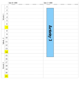 Exhibit 2: Single activity at a single location |
 Exhibit 3: Staggered activity |
 Exhibit 4: Parallelogram activity |
 Exhibit 5: Non-linear activity |
 Exhibit 6: Activities with no-work periods |
Tools
Time–distance diagrams can be created using any kind of drawing tool, certainly one which allows scaled drawing (for example, CAD editors, Visio). Sometimes, spreadsheet tools are employed where the width of the columns and the height of the rows form the distance and time scales.
However, in real project life, a time schedule needs to be adjusted continuously: This is when the use of specialized tools quickly brings out their advantage. These tools (see External links below) are project management tools in their own right with an emphasis on the ability to present the time schedule as time–distance diagram. Activities can be edited using project management terminology plus all drawing attributes for the activity's shape. Special features allow dependency links (with lags), complex scaling, access conflict detection, resource-dependent progress, and more. Most often, such tools provide various interfaces to other project management software, at least to import and export activity information. Complex systems (such as TimeChainage, DynaRoad, TILOS or Time Location Plus) even integrate into commonly used project management software (Primavera, Microsoft Project, Asta Powerproject).
See also
- Linear scheduling method
- Project management
- Project planning
- Service planning (train)
- List of project management topics
- List of project management software
References
- Aeroplane and commercial aviation news, Volume 87, 1954
- Chakroborty, Partha; Das, Animesh (2004). Principles of Transportation Engineering. PHI Learning Pvt. Ltd. p. 89.
- Gallo, M.; D'Acieerno, L.; Montella, B. (2011). A multimodal approach to bus frequency design. Urban Transport XVII: Urban Transport and the Environment in the 21st Century. 116. WIT Press. p. 220.
- Emmitt, Stephen (2007). Design management for architects. Wiley-Blackwell. p. 97. ISBN 978-1-4051-3147-6.
- Federal Transit Administration, Honolulu High-Capacity Transit Corridor Project Report, July 2009 (Final), figure 4-1 on page 4-10
- http://topconplanning.com/kb/article/374/control-of-a-large-scale-tunnel-project
External links
| Wikimedia Commons has media related to Time–distance diagram. |
- TILOS: Linear project GmbH, Germany (with many examples
- Turbo Chart: Linear Project Software Pty Ltd, Australia
- GraphicSchedule, an Excel application: www.GraphicSchedule.com
- ChainLink: Steven Wood Software, United Kingdom
- TimeChainage: Peter Milton Planning, United Kingdom
- DynaRoad: DynaRoad Ltd., Finland
- LinearPlus: PCF Ltd., United Kingdom
- Planisfer: Mire S.A.S, France
from projects using time-distance diagrams)
- Time Location Plus: Naylor Computing, United Kingdom
- Vico Office: Vico Software, Inc., USA
Further reading
- James Wonneberg and Ron Drake (2016) Linear Scheduling 101
- Austen, A. D.; Neale, R. H. (1984). Managing construction projects: a guide to processes and procedures. International Labour Organization. p. 110ff. ISBN 978-92-2-106476-3.
- CIOB (Chartered Institute of Building) (2011). Guide to Good Practice in the Management of Time in Complex Projects. John Wiley and Sons. ISBN 978-1-4443-3493-7.
- Cooke, Brian; Williams, Peter (2004). Construction planning, programming, and control (2nd ed.). Blackwell Publishing Ltd. ISBN 978-1-4051-2148-4.
- Hamilton, Albert (2001). Managing projects for success: a trilogy. Thomas Telford. ISBN 978-0-7277-3497-6.
- Neale, R. H.; Neale, David E. (1989). Construction planning. Engineering management. Thomas Telford. p. 44ff. ISBN 978-0-7277-1322-3.