Successive over-relaxation

Given a square system of n linear equations with unknown x:

${\displaystyle A\mathbf {x} =\mathbf {b} }$

where:

${\displaystyle A={\begin{bmatrix}a_{11}&a_{12}&\cdots &a_{1n}\\a_{21}&a_{22}&\cdots &a_{2n}\\\vdots &\vdots &\ddots &\vdots \\a_{n1}&a_{n2}&\cdots &a_{nn}\end{bmatrix}},\qquad \mathbf {x} ={\begin{bmatrix}x_{1}\\x_{2}\\\vdots \\x_{n}\end{bmatrix}},\qquad \mathbf {b} ={\begin{bmatrix}b_{1}\\b_{2}\\\vdots \\b_{n}\end{bmatrix}}.}$

Then A can be decomposed into a diagonal component D, and strictly lower and upper triangular components L and U:

${\displaystyle A=D+L+U,}$

where

${\displaystyle D={\begin{bmatrix}a_{11}&0&\cdots &0\\0&a_{22}&\cdots &0\\\vdots &\vdots &\ddots &\vdots \\0&0&\cdots &a_{nn}\end{bmatrix}},\quad L={\begin{bmatrix}0&0&\cdots &0\\a_{21}&0&\cdots &0\\\vdots &\vdots &\ddots &\vdots \\a_{n1}&a_{n2}&\cdots &0\end{bmatrix}},\quad U={\begin{bmatrix}0&a_{12}&\cdots &a_{1n}\\0&0&\cdots &a_{2n}\\\vdots &\vdots &\ddots &\vdots \\0&0&\cdots &0\end{bmatrix}}.}$

The system of linear equations may be rewritten as:

${\displaystyle (D+\omega L)\mathbf {x} =\omega \mathbf {b} -[\omega U+(\omega -1)D]\mathbf {x} }$

for a constant ω > 1, called the relaxation factor.

The method of successive over-relaxation is an iterative technique that solves the left hand side of this expression for x, using previous value for x on the right hand side. Analytically, this may be written as:

${\displaystyle \mathbf {x} ^{(k+1)}=(D+\omega L)^{-1}{\big (}\omega \mathbf {b} -[\omega U+(\omega -1)D]\mathbf {x} ^{(k)}{\big )}=L_{w}\mathbf {x} ^{(k)}+\mathbf {c} ,}$

where ${\displaystyle \mathbf {x} ^{(k)}}$ is the kth approximation or iteration of ${\displaystyle \mathbf {x} }$ and ${\displaystyle \mathbf {x} ^{(k+1)}}$ is the next or k + 1 iteration of ${\displaystyle \mathbf {x} }$. However, by taking advantage of the triangular form of (D+ωL), the elements of x^(k+1) can be computed sequentially using forward substitution:

${\displaystyle x_{i}^{(k+1)}=(1-\omega )x_{i}^{(k)}+{\frac {\omega }{a_{ii}}}\left(b_{i}-\sum _{j<i}a_{ij}x_{j}^{(k+1)}-\sum _{j>i}a_{ij}x_{j}^{(k)}\right),\quad i=1,2,\ldots ,n.}$

Spectral radius ${\displaystyle \rho (C_{\omega })}$ of the iteration matrix for the SOR method ${\displaystyle C_{\omega }}$. The plot shows the dependence on the spectral radius of the Jacobi iteration matrix ${\displaystyle \mu$ :=\rho (C_{\text{Jac}})} .

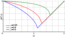
The choice of relaxation factor ω is not necessarily easy, and depends upon the properties of the coefficient matrix. In 1947, Ostrowski proved that if ${\displaystyle A}$ is symmetric and positive-definite then ${\displaystyle \rho (L_{\omega })<1}$ for ${\displaystyle 0<\omega <2}$. Thus, convergence of the iteration process follows, but we are generally interested in faster convergence rather than just convergence.

Since elements can be overwritten as they are computed in this algorithm, only one storage vector is needed, and vector indexing is omitted. The algorithm goes as follows:

Inputs: A, b, ω
Output: ${\displaystyle \phi }$

Choose an initial guess ${\displaystyle \phi }$ to the solution
repeat until convergence
    for i from 1 until n do
        ${\displaystyle \sigma \leftarrow 0}$
        for j from 1 until n do
            if j ≠ i then
                ${\displaystyle \sigma \leftarrow \sigma +a_{ij}\phi _{j}}$
            end if
        end (j-loop)
        ${\displaystyle \phi _{i}\leftarrow (1-\omega )\phi _{i}+{\frac {\omega }{a_{ii}}}(b_{i}-\sigma )}$
    end (i-loop)
    check if convergence is reached
end (repeat)

Note

${\displaystyle (1-\omega )\phi _{i}+{\frac {\omega }{a_{ii}}}(b_{i}-\sigma )}$ can also be written ${\displaystyle \phi _{i}+\omega \left({\frac {b_{i}-\sigma }{a_{ii}}}-\phi _{i}\right)}$, thus saving one multiplication in each iteration of the outer for-loop.

We are presented the linear system

${\displaystyle {\begin{aligned}4x_{1}-x_{2}-6x_{3}+0x_{4}=2,\\-5x_{1}-4x_{2}+10x_{3}+8x_{4}=21,\\0x_{1}+9x_{2}+4x_{3}-2x_{4}=-12,\\1x_{1}+0x_{2}-7x_{3}+5x_{4}=-6.\end{aligned}}}$

To solve the equations, we choose a relaxation factor ${\displaystyle \omega =0.5}$ and an initial guess vector ${\displaystyle \phi =(0,0,0)}$. According to the successive over-relaxation algorithm, following table is obtained, representing an exemplary iteration with approximations, which ideally, but not necessarily, finds the exact solution, (3, −2, 2, 1), in 38 steps.

Iteration	${\displaystyle x_{1}}$	${\displaystyle x_{2}}$	${\displaystyle x_{3}}$	${\displaystyle x_{4}}$
1	0.25	-2.78125	1.6289062	0.5152344
2	1.2490234	-2.2448974	1.9687712	0.9108547
3	2.070478	-1.6696789	1.5904881	0.76172125
...	...	...	...	...
37	2.9999998	-2.0	2.0	1.0
38	3.0	-2.0	2.0	1.0

A simple implementation of the algorithm in Common Lisp is offered below. Beware its proclivity towards floating-point overflows in the general case.

(defparameter +MAXIMUM-NUMBER-OF-ITERATIONS+ 100
  "The number of iterations beyond which the algorithm should
   cease its operation, regardless of its current solution.")

(defun get-errors (computed-solution exact-solution)
  "For each component of the COMPUTED-SOLUTION vector, retrieves its
   error with respect to the expected EXACT-SOLUTION, returning a
   vector of error values."
  (map 'vector #'- exact-solution computed-solution))

(defun is-convergent (errors &key (error-tolerance 0.001))
  "Checks whether the convergence is reached with respect to the
   ERRORS vector which registers the discrepancy betwixt the computed
   and the exact solution vector.
   ---
   The convergence is fulfilled iff each absolute error component is
   less than or equal to the ERROR-TOLERANCE."
  (flet ((error-is-acceptable (error)
          (<= (abs error) error-tolerance)))
    (every #'error-is-acceptable errors)))

(defun make-zero-vector (size)
  "Creates and returns a vector of the SIZE with all elements set to 0."
  (make-array size :initial-element 0.0 :element-type 'number))

(defun sor (A b omega
            &key (phi (make-zero-vector (length b)))
                 (convergence-check
                   #'(lambda (iteration phi)
                       (declare (ignore phi))
                       (>= iteration +MAXIMUM-NUMBER-OF-ITERATIONS+))))
  "Implements the successive over-relaxation (SOR) method, applied upon
   the linear equations defined by the matrix A and the right-hand side
   vector B, employing the relaxation factor OMEGA, returning the
   calculated solution vector.
   ---
   The first algorithm step, the choice of an initial guess PHI, is
   represented by the optional keyword parameter PHI, which defaults
   to a zero-vector of the same structure as B. If supplied, this
   vector will be destructively modified. In any case, the PHI vector
   constitutes the function's result value.
   ---
   The terminating condition is implemented by the CONVERGENCE-CHECK,
   an optional predicate
     lambda(iteration phi) => generalized-boolean
   which returns T, signifying the immediate termination, upon achieving
   convergence, or NIL, signaling continuant operation, otherwise."
  (let ((n (array-dimension A 0)))
    (loop for iteration from 1 by 1 do
      (loop for i from 0 below n by 1 do
        (let ((rho 0))
          (loop for j from 0 below n by 1 do
            (when (/= j i)
              (let ((a[ij]  (aref A i j))
                    (phi[j] (aref phi j)))
                (incf rho (* a[ij] phi[j])))))
          (setf (aref phi i)
                (+ (* (- 1 omega)
                      (aref phi i))
                   (* (/ omega (aref A i i))
                      (- (aref b i) rho))))))
      (format T "~&~d. solution = ~a" iteration phi)
      ;; Check if convergence is reached.
      (when (funcall convergence-check iteration phi)
        (return))))
  phi)

;; Summon the function with the exemplary parameters.
(let ((A              (make-array (list 4 4)
                        :initial-contents
                        '((  4  -1  -6   0 )
                          ( -5  -4  10   8 )
                          (  0   9   4  -2 )
                          (  1   0  -7   5 ))))
      (b              (vector 2 21 -12 -6))
      (omega          0.5)
      (exact-solution (vector 3 -2 2 1)))
  (sor
    A b omega
    :convergence-check
    #'(lambda (iteration phi)
        (let ((errors (get-errors phi exact-solution)))
          (format T "~&~d. errors   = ~a" iteration errors)
          (or (is-convergent errors :error-tolerance 0.0)
              (>= iteration +MAXIMUM-NUMBER-OF-ITERATIONS+))))))

A simple Python implementation of the pseudo-code provided above.

import numpy as np

def sor_solver(A, b, omega, initial_guess, convergence_criteria):
    """
    This is an implementation of the pseudo-code provided in the Wikipedia article.
    Arguments:
        A: nxn numpy matrix.
        b: n dimensional numpy vector.
        omega: relaxation factor.
        initial_guess: An initial solution guess for the solver to start with.
        convergence_criteria: The maximum discrepancy acceptable to regard the current solution as fitting.
    Returns:
        phi: solution vector of dimension n.
    """
    phi = initial_guess[:]
    residual = np.linalg.norm(np.matmul(A, phi) - b) #Initial residual
    while residual > convergence_criteria:
        for i in range(A.shape[0]):
            sigma = 0
            for j in range(A.shape[1]):
                if j != i:
                    sigma += A[i][j] * phi[j]
            phi[i] = (1 - omega) * phi[i] + (omega / A[i][i]) * (b[i] - sigma)
        residual = np.linalg.norm(np.matmul(A, phi) - b)
        print('Residual: {0:10.6g}'.format(residual))
    return phi


# An example case that mirrors the one in the Wikipedia article
residual_convergence = 1e-8
omega = 0.5 #Relaxation factor

A = np.matrix([4, -1, -6, 0],
              [-5, -4, 10, 8],
              [0, 9, 4, -2],
              [1, 0, -7, 5])

b = np.matrix([2, 21, -12, -6])

initial_guess = np.zeros(4)

phi = sor_solver(A, b, omega, initial_guess, residual_convergence)
print(phi)

The version for symmetric matrices A, in which

${\displaystyle U=L^{T},\,}$

is referred to as Symmetric Successive Over-Relaxation, or (SSOR), in which

${\displaystyle P=\left({\frac {D}{\omega }}+L\right){\frac {\omega }{2-\omega }}D^{-1}\left({\frac {D}{\omega }}+U\right),}$

and the iterative method is

${\displaystyle \mathbf {x} ^{k+1}=\mathbf {x} ^{k}-\gamma ^{k}P^{-1}(A\mathbf {x} ^{k}-\mathbf {b} ),\ k\geq 0.}$

The SOR and SSOR methods are credited to David M. Young, Jr..

A similar technique can be used for any iterative method. If the original iteration had the form

${\displaystyle x_{n+1}=f(x_{n})}$

then the modified version would use

${\displaystyle x_{n+1}^{\mathrm {SOR} }=(1-\omega )x_{n}^{\mathrm {SOR} }+\omega f(x_{n}^{\mathrm {SOR} }).}$

However, the formulation presented above, used for solving systems of linear equations, is not a special case of this formulation if x is considered to be the complete vector. If this formulation is used instead, the equation for calculating the next vector will look like

${\displaystyle \mathbf {x} ^{(k+1)}=(1-\omega )\mathbf {x} ^{(k)}+\omega L_{*}^{-1}(\mathbf {b} -U\mathbf {x} ^{(k)}),}$

where ${\displaystyle L_{*}=L+D}$. Values of ${\displaystyle \omega >1}$ are used to speed up convergence of a slow-converging process, while values of ${\displaystyle \omega <1}$ are often used to help establish convergence of a diverging iterative process or speed up the convergence of an overshooting process.

There are various methods that adaptively set the relaxation parameter ${\displaystyle \omega }$ based on the observed behavior of the converging process. Usually they help to reach a super-linear convergence for some problems but fail for the others.

• Jacobi method
• Gaussian Belief Propagation
• Matrix splitting

• This article incorporates text from the article Successive_over-relaxation_method_-_SOR on CFD-Wiki that is under the GFDL license.

• Abraham Berman, Robert J. Plemmons, Nonnegative Matrices in the Mathematical Sciences, 1994, SIAM. ISBN 0-89871-321-8.
• Black, Noel and Moore, Shirley. "Successive Overrelaxation Method". MathWorld.CS1 maint: multiple names: authors list (link)
• A. Hadjidimos, Successive overrelaxation (SOR) and related methods, Journal of Computational and Applied Mathematics 123 (2000), 177-199.
• Yousef Saad, Iterative Methods for Sparse Linear Systems, 1st edition, PWS, 1996.
• Netlib's copy of "Templates for the Solution of Linear Systems", by Barrett et al.
• Richard S. Varga 2002 Matrix Iterative Analysis, Second ed. (of 1962 Prentice Hall edition), Springer-Verlag.
• David M. Young, Jr. Iterative Solution of Large Linear Systems, Academic Press, 1971. (reprinted by Dover, 2003)

• Module for the SOR Method
• Tridiagonal linear system solver based on SOR, in C++