Smallest-circle problem
The smallest-circle problem (also known as minimum covering circle problem, bounding circle problem, smallest enclosing circle problem) is a mathematical problem of computing the smallest circle that contains all of a given set of points in the Euclidean plane. The corresponding problem in n-dimensional space, the smallest bounding sphere problem, is to compute the smallest n-sphere that contains all of a given set of points.[1] The smallest-circle problem was initially proposed by the English mathematician James Joseph Sylvester in 1857.[2]
The smallest-circle problem in the plane is an example of a facility location problem (the 1-center problem) in which the location of a new facility must be chosen to provide service to a number of customers, minimizing the farthest distance that any customer must travel to reach the new facility.[3] Both the smallest circle problem in the plane, and the smallest bounding sphere problem in any higher-dimensional space of bounded dimension are solvable in worst-case linear time.
Characterization
Most of the geometric approaches for the problem look for points that lie on the boundary of the minimum circle and are based on the following simple facts:
- The minimum covering circle is unique.
- The minimum covering circle of a set S can be determined by at most three points in S which lie on the boundary of the circle. If it is determined by only two points, then the line segment joining those two points must be a diameter of the minimum circle. If it is determined by three points, then the triangle consisting of those three points is not obtuse.
Proof that the minimum covering disk is unique |
|---|
|
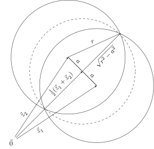
Let P be any set of points in the plane, and suppose that there are two smallest enclosing disks of P, with centers at and . Let be their shared radius, and let be the distance between their centers. Since P is a subset of both disks it is a subset of their intersection. However, their intersection is contained within the disk with center and radius , as shown in the following image: Since r is minimal, we must have , meaning , so the disks are identical.[4] |


Linear-time solutions
As Nimrod Megiddo showed,[5] the minimum enclosing circle can be found in linear time, and the same linear time bound also applies to the smallest enclosing sphere in Euclidean spaces of any constant dimension. His article also gives a brief overview of earlier O(n^3) and O(n log n) algorithms.[6]
Emo Welzl[7] proposed a simple randomized algorithm for the minimum covering circle problem that runs in expected time , based on a linear programming algorithm of Raimund Seidel.

Subsequently, the smallest-circle problem was included in a general class of LP-type problems that can be solved by algorithms like Welzl's based on linear programming. As a consequence of membership in this class, it was shown that the dependence on the dimension of the constant factor in the time bound, which was factorial for Seidel's method, could be reduced to subexponential.[6]
Megiddo's algorithm

Megiddo's algorithm[8] is based on the technique called prune and search reducing size of the problem by removal of n/16 of unnecessary points. That leads to the recurrence t(n)≤ t(15n/16)+cn giving t(n)=16cn.
The algorithm is rather complicated and it is reflected in big multiplicative constant. The reduction needs to solve twice the similar problem where center of the sought-after enclosing circle is constrained to lie on a given line. The solution of the subproblem is either solution of unconstrained problem or it is used to determine the half-plane where the unconstrained solution center is located.
The n/16 points to be discarded are found the following way: Points Pi are arranged to pairs what defines n/2 lines pj as their bisectors. Median pm of bisectors in order by their directions (oriented to the same half-plane determined by bisector p1) is found and pairs from bisectors are made, such that in each pair one bisector has direction at most pm and the other at least pm (direction p1 could be considered as - or + according our needs.) Let Qk be intersection of bisectors of k-th pair.

Line q in the p1 direction is placed to go through an intersection Qx such that there is n/8 intersections in each half-plane defined by the line (median position). Constrained version of the enclosing problem is run on line q what determines half-plane where the center is located. Line q' in the pm direction is placed to go through an intersection Qx' such that there is n/16 intersections in each half of the half-plane not containing the solution. Constrained version of the enclosing problem is run on line q' what together with q determines quadrant, where the center is located. We consider the points Qk in the quadrant not contained in a half-plane containing solution. One of the bisectors of pair defining Qk has the direction ensuring which of points Pi defining the bisector is closer to each point in the quadrant containing the center of the enclosing circle. This point could be discarded.
The constrained version of the algorithm is also solved by the prune and search technique, but reducing problem size by removal of n/4 points leading to recurrence t(n)≤ t(3n/4)+cn giving t(n)=4cn.
The n/4 points to be discarded are found the following way: Points Pi are arranged to pairs. For each pair intersection Qj of its bisector with the constraining line q is found. (If intersection does not exist we could remove one point from the pair immediately). Median M of points Qj on the line q is found and in O(n) time is determined which halfline of q starting in M contains the solution of the constrained problem. We consider points Qj from the other half. We know which of points Pi defining Qj is closer to the each point of the halfline containing center of the enclosing circle of the constrained problem solution. This point could be discarded.
The half-plane where the unconstrained solution lies could be determined by the points Pi on the boundary of the constrained circle solution. (First and last point on the circle in each half-plane suffice. If the center belongs to their convex hull, it is unconstrained solution, otherwise direction to the nearest edge determines half-plane of the unconstrained solution.)
Welzl's algorithm
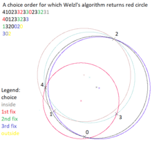
Welzl described the algorithm in a recursive form. For size of input set at most 3, trivial algorithm is created. It outputs empty circle, circle with radius 0, circle on diameter made by arc of input points for input sizes 0, 1 and 2 respectively. For input size 3 if the points are vertices of an acute triangle, the circumscribed circle is returned. Otherwise the circle having a diameter of the triangle's longest edge is returned. For bigger sizes the algorithm uses solution of 1 smaller size where the ignored point p is chosen randomly and uniformly. The returned circle D is checked and if it encloses p, it is returned as result. Otherwise we know point p is on border of the result. We rerun the algorithm again, but we call it with the information p is on the result circle boundary. Points which are known to be on the boundary are accumulated in the set R and they are excluded from the subset P from which random choices are made in the following calls.
The condition to use the trivial algorithm is |P|=0 or |R|=3, and the trivial algorithm is called for R. Equivalent condition would be |R|=3 or |P|+|R|≤3, and call of the trivial algorithm for R in the case |R|=3 and for union of P and R otherwise. This would prevent some recursive calls on bottom of the recursion.
algorithm welzl is[7]
    input: Finite sets P and R of points in the plane |R|≤ 3.
    output: Minimal disk enclosing P with R on the boundary.
    if P is empty or |R| = 3 then
        return trivial(R)
    choose p in P (randomly and uniformly)
    D := welzl(P - { p }, R)
    if p is in D then
        return D
    return welzl(P - { p }, R ∪ { p })
Welzl indicated implementation without need of recursion. Empty R and random permutation of P is used at start. Sets on bottom of recursion correspond to prefixes in the permutation. Trivial algorithm is called for R extended by prefix of P to size of 3, and following points are checked they are enclosed by its result D. Whenever check fails on point p, p is added to R and removed from P, and the prefix of the permutation up to p is reshufled. To make this implementation equivalent to the recursive one, we should maintain stack of prefix lengths and if longer prefix than the top would be inserted, last point from R should be removed and inserted to P, the top prefix on the stack should be removed at the same time. Therefore, the prefix length on stack would be nondecreasing from its top down. When |R|=3, the points up to prefix length on top position of the stack are not checked.
Typical implementation uses one list(array) of points of R ∪ P with R in its start, remembering the size of R, therefore sizeR could be used as stack pointer and its decrements while top prefix length was smaller than the current prefix length to be inserted does all required actions.
Welzl also proposes functionally different version of the algorithm using random permutation of points on input, where the points are not reshuffled when the point p is moved to front of the list. The algorithm is again presented in the recursive form.
Matoušek, Sharir, Welzl's algorithm
Matoušek, Sharir, Welzl [6] implicitly warned that the assumption point moved to R remains on enclosing circle's boundary for all subsets of R ∪ P does not hold, and the required additional condition is the radius of the enclosing circle does not decrease.
They proposed tiny change to the algorithm forcing the radius of the enclosing circle does not decrease. If p is not in enclosing circle D of R ∪ P - { p }, the radius r of enclosing circle of D must be smaller than radius r' of enclosing circle D' of R ∪ P. But radius of an enclosing circle of any subset of R ∪ P - { p } is at most r, so whenever r*>r is radius of an enclosing circle of a subset of R ∪ P, p must be in its boundary.
MSW algorithm chooses 3 random points of P as initial base R and they find initial D by running the trivial algorithm on them. The presented recursive version of the algorithm is very similar to Welzl's. Point p of P is chosen in random order and algorithm for the set P - { p } is called. If p is not enclosed by returned circle D, p replaces one of 3 points in the base (R ∪ P does not change, and |R| remains 3), such that the enclosing circle of the new base encloses the point removed from the base. The result recursion is restarted with changed P, R.
algorithm msw is
    input: Finite sets P and R of points in the plane |R|=3
    output: Minimal disk enclosing P ∪ R
    if P is empty then
        return trivial(R)
    choose p in P (randomly and uniformly)
    D := msw(P - { p }, R)
    if p is in D then
        return D
    q := nonbase(R ∪ { p }) (Welzl's algorithm for 4 points could be used to find what would not be in R)
    return msw(P - { p } ∪ { q }, R ∪ { p } - { q })
Use of base extended by one point is mentioned in the paper. If we put p to the extended base replacing extension, we could use Welzl's recurrence to rearrange the extended base to base and the extra point. You can look at it as allowing temporary decrease of radius r which would be restored when the extended base is finished. The move to front version of Welzl's algorithm works according to this schema except the randomization of choices. This is why it returns correct results, on the contrary to the Welzl's original algorithm.
Move to front version of welzl without recursion and one list for R ∪ P in view of msw algorithm could be simplified by not maintaining the size of R at all.
Experiments indicate the move to front version have performance slightly better (say 2% less checks p belongs to D) than the rerandomized one (of msw).
Other algorithms
Prior to Megiddo's result showing that the smallest-circle problem may be solved in linear time, several algorithms of higher complexity appeared in the literature. A naive algorithm solves the problem in time O(n4) by testing the circles determined by all pairs and triples of points.
- An algorithm of Chrystal and Peirce applies a local optimization strategy that maintains two points on the boundary of an enclosing circle and repeatedly shrinks the circle, replacing the pair of boundary points, until an optimal circle is found. Chakraborty and Chaudhuri[9] propose a linear-time method for selecting a suitable initial circle and a pair of boundary points on that circle. Each step of the algorithm includes as one of the two boundary points a new vertex of the convex hull, so if the hull has h vertices this method can be implemented to run in time O(nh).
- Elzinga and Hearn[10] described an algorithm which maintains a covering circle for a subset of the points. At each step, a point not covered by the current sphere is used to find a larger sphere that covers a new subset of points, including the point found. Although its worst case running time is O(h3n), the authors report that it ran in linear time in their experiments. The complexity of the method has been analyzed by Drezner and Shelah.[11] Both Fortran and C codes are available from Hearn, Vijay & Nickel (1995).[12]
- The smallest sphere problem can be formulated as a quadratic program[1] defined by a system of linear constraints with a convex quadratic objective function. Therefore, any feasible direction algorithm can give the solution of the problem.[13] Hearn and Vijay[14] proved that the feasible direction approach chosen by Jacobsen is equivalent to the Chrystal–Peirce algorithm.
- The dual to this quadratic program may also be formulated explicitly;[15] an algorithm of Lawson[16] can be described in this way as a primal dual algorithm.[14]
- Shamos and Hoey[17] proposed an O(n log n) time algorithm for the problem based on the observation that the center of the smallest enclosing circle must be a vertex of the farthest-point Voronoi diagram of the input point set.
Weighted variants of the problem
The weighted version of the minimum covering circle problem takes as input a set of points in a Euclidean space, each with weights; the goal is to find a single point that minimizes the maximum weighted distance to any point. The original minimum covering circle problem can be recovered by setting all weights to the same number. As with the unweighted problem, the weighted problem may be solved in linear time in any space of bounded dimension, using approaches closely related to bounded dimension linear programming algorithms, although slower algorithms are again frequent in the literature.[14][18][19]
References
- Elzinga, J.; Hearn, D. W. (1972), "The minimum covering sphere problem", Management Science, 19: 96–104, doi:10.1287/mnsc.19.1.96
- Sylvester, J. J. (1857), "A question in the geometry of situation", Quarterly Journal of Mathematics, 1: 79.
- Francis, R. L.; McGinnis, L. F.; White, J. A. (1992), Facility Layout and Location: An Analytical Approach (2nd ed.), Englewood Cliffs, N.J.: Prentice–Hall, Inc..
- Welzl 1991, p. 2.
- Megiddo, Nimrod (1983), "Linear-time algorithms for linear programming in R3 and related problems", SIAM Journal on Computing, 12 (4): 759–776, doi:10.1137/0212052, MR 0721011.
- Matoušek, Jiří; Sharir, Micha; Welzl, Emo (1996), "A subexponential bound for linear programming" (PDF), Algorithmica, 16 (4–5): 498–516, CiteSeerX 10.1.1.46.5644, doi:10.1007/BF01940877.
- Welzl, Emo (1991), "Smallest enclosing disks (balls and ellipsoids)", in Maurer, H. (ed.), New Results and New Trends in Computer Science, Lecture Notes in Computer Science, 555, Springer-Verlag, pp. 359–370, CiteSeerX 10.1.1.46.1450, doi:10.1007/BFb0038202, ISBN 978-3-540-54869-0.
- Megiddo, Nimrod (1983), "Linear-time algorithms for linear programming in R3 and related problems", SIAM Journal on Computing, 12 (4): 759–776, doi:10.1137/0212052, MR 0721011.
- Chakraborty, R. K.; Chaudhuri, P. K. (1981), "Note on geometrical solutions for some minimax location problems", Transportation Science, 15 (2): 164–166, doi:10.1287/trsc.15.2.164.
- Elzinga, J.; Hearn, D. W. (1972), "Geometrical solutions for some minimax location problems", Transportation Science, 6 (4): 379–394, doi:10.1287/trsc.6.4.379.
- Drezner, Z.; Shelah, S. (1987), "On the complexity of the Elzinga–Hearn algorithm for the 1-center problem", Mathematics of Operations Research, 12 (2): 255–261, doi:10.1287/moor.12.2.255, JSTOR 3689688.
- Hearn, D. W.; Vijay, J.; Nickel, S. (1995), "Codes of geometrical algorithms for the (weighted) minimum circle problem", European Journal of Operational Research, 80: 236–237, doi:10.1016/0377-2217(95)90075-6.
- Jacobsen, S. K. (1981), "An algorithm for the minimax Weber problem", European Journal of Operational Research, 6 (2): 144–148, doi:10.1016/0377-2217(81)90200-9.
- Hearn, D. W.; Vijay, J. (1982), "Efficient algorithms for the (weighted) minimum circle problem", Operations Research, 30 (4): 777–795, doi:10.1287/opre.30.4.777.
- Elzinga, J.; Hearn, D. W.; Randolph, W. D. (1976), "Minimax multifacility location with Euclidean distances", Transportation Science, 10 (4): 321–336, doi:10.1287/trsc.10.4.321.
- Lawson, C. L. (1965), "The smallest covering cone or sphere", SIAM Review, 7 (3): 415–417, doi:10.1137/1007084.
- Shamos, M. I.; Hoey, D. (1975), "Closest point problems", Proceedings of 16th Annual IEEE Symposium on Foundations of Computer Science, pp. 151–162, doi:10.1109/SFCS.1975.8.
- Megiddo, N. (1983), "The weighted Euclidean 1-center problem", Mathematics of Operations Research, 8 (4): 498–504, doi:10.1287/moor.8.4.498.
- Megiddo, N.; Zemel, E. (1986), "An O(n log n) randomizing algorithm for the weighted Euclidean 1-center problem", Journal of Algorithms, 7 (3): 358–368, doi:10.1016/0196-6774(86)90027-1.
External links
- Bernd Gärtner's smallest enclosing ball code
- CGAL the Min_sphere_of_spheres package of the Computational Geometry Algorithms Library (CGAL)
- Miniball an open-source implementation of an algorithm for the smallest enclosing ball problem for low and moderately high dimensions