Simpson's paradox
Simpson's paradox, which goes by several names, is a phenomenon in probability and statistics, in which a trend appears in several different groups of data but disappears or reverses when these groups are combined. This result is often encountered in social-science and medical-science statistics[1][2][3] and is particularly problematic when frequency data is unduly given causal interpretations.[4] The paradox can be resolved when causal relations are appropriately addressed in the statistical modeling.[4][5]

Simpson's paradox has been used as an exemplar to illustrate to the non-specialist or public audience the kind of misleading results mis-applied statistics can generate.[6][7] Martin Gardner wrote a popular account of Simpson's paradox in his March 1976 Mathematical Games column in Scientific American.[8]
Edward H. Simpson first described this phenomenon in a technical paper in 1951,[9] but the statisticians Karl Pearson et al., in 1899,[10] and Udny Yule, in 1903,[11] had mentioned similar effects earlier. The name Simpson's paradox was introduced by Colin R. Blyth in 1972.[12]
It is also referred to as or Simpson's reversal, Yule–Simpson effect, amalgamation paradox, or reversal paradox.[13]
Examples
UC Berkeley gender bias
One of the best-known examples of Simpson's paradox is a study of gender bias among graduate school admissions to University of California, Berkeley. The admission figures for the fall of 1973 showed that men applying were more likely than women to be admitted, and the difference was so large that it was unlikely to be due to chance.[14][15]
| Men | Women | |||
|---|---|---|---|---|
| Applicants | Admitted | Applicants | Admitted | |
| Total | 8442 | 44% | 4321 | 35% |
However, when examining the individual departments, it appeared that six out of 85 departments were significantly biased against men, whereas four were significantly biased against women. In fact, the pooled and corrected data showed a "small but statistically significant bias in favor of women".[15] The data from the six largest departments are listed below, the top two departments by number of applicants for each gender italicised.
| Department | Men | Women | ||
|---|---|---|---|---|
| Applicants | Admitted | Applicants | Admitted | |
| A | 825 | 62% | 108 | 82% |
| B | 560 | 63% | 25 | 68% |
| C | 325 | 37% | 593 | 34% |
| D | 417 | 33% | 375 | 35% |
| E | 191 | 28% | 393 | 24% |
| F | 373 | 6% | 341 | 7% |
The research paper by Bickel et al.[15] concluded that women tended to apply to competitive departments with low rates of admission even among qualified applicants (such as in the English Department), whereas men tended to apply to less-competitive departments with high rates of admission among the qualified applicants (such as in engineering and chemistry).
Kidney stone treatment
This is a real-life example from a medical study[16] comparing the success rates of two treatments for kidney stones.[17]
The table below shows the success rates and numbers of treatments for treatments involving both small and large kidney stones, where Treatment A includes all open surgical procedures and Treatment B is percutaneous nephrolithotomy (which involves only a small puncture). The numbers in parentheses indicate the number of success cases over the total size of the group.
Treatment Stone size |
Treatment A | Treatment B |
|---|---|---|
| Small stones | Group 1 93% (81/87) | Group 2 87% (234/270) |
| Large stones | Group 3 73% (192/263) | Group 4 69% (55/80) |
| Both | 78% (273/350) | 83% (289/350) |
The paradoxical conclusion is that treatment A is more effective when used on small stones, and also when used on large stones, yet treatment B is more effective when considering both sizes at the same time. In this example, the "lurking" variable (or confounding variable) is the severity of the case (represented by the doctors' treatment decision trend of favoring B for less severe cases), which was not previously known to be important until its effects were included.
Which treatment is considered better is determined by an inequality between two ratios (successes/total). The reversal of the inequality between the ratios, which creates Simpson's paradox, happens because two effects occur together:
- The sizes of the groups, which are combined when the lurking variable is ignored, are very different. Doctors tend to give the severe cases (large stones) the better treatment (A), and the milder cases (small stones) the inferior treatment (B). Therefore, the totals are dominated by groups 3 and 2, and not by the two much smaller groups 1 and 4.
- The lurking variable has a large effect on the ratios; i.e., the success rate is more strongly influenced by the severity of the case than by the choice of treatment. Therefore, the group of patients with large stones using treatment A (group 3) does worse than the group with small stones (groups 1 and 2), even if the latter used the inferior treatment B (group 2).
Based on these effects, the paradoxical result is seen to arise by suppression of the causal effect of the severity of the case on successful treatment. The paradoxical result can be rephrased more accurately as follows: When the less effective treatment (B) is applied more frequently to less severe cases, it can appear to be a more effective treatment.
Batting averages
A common example of Simpson's paradox involves the batting averages of players in professional baseball. It is possible for one player to have a higher batting average than another player each year for a number of years, but to have a lower batting average across all of those years. This phenomenon can occur when there are large differences in the number of at bats between the years. Mathematician Ken Ross[18] demonstrated this using the batting average of two baseball players, Derek Jeter and David Justice, during the years 1995 and 1996:[19]
Year Batter |
1995 | 1996 | Combined | |||
|---|---|---|---|---|---|---|
| Derek Jeter | 12/48 | .250 | 183/582 | .314 | 195/630 | .310 |
| David Justice | 104/411 | .253 | 45/140 | .321 | 149/551 | .270 |
In both 1995 and 1996, Justice had a higher batting average (in bold type) than Jeter did. However, when the two baseball seasons are combined, Jeter shows a higher batting average than Justice. According to Ross, this phenomenon would be observed about once per year among the possible pairs of players.
Racial disparity in the death penalty
This real-life example is taken from Radelet.[20] The data are from twenty Florida counties during 1976-1977.
Defendant Victim |
White | Black | Both |
|---|---|---|---|
| White | 13% (19/151) | 17% (11/63) | 14% (30/214) |
| Black | 0% (0/9) | 6% (6/103) | 5% (6/112) |
| Both | 12% (19/160) | 10% (17/166) |
When disaggregating the data by the race of the victim, it appears that black defendants are more likely to be sentenced to the death penalty. However, since most victims are white, crimes against white victims have higher sentencing rates, and most of the crimes against white victims were committed by white defendants, the aggregate data indicates that white defendants are more likely to be sentenced to the death penalty.
Vector interpretation

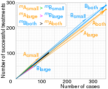
Simpson's paradox can also be illustrated using the 2-dimensional vector space.[21] A success rate of (i.e., successes/attempts) can be represented by a vector , with a slope of . A steeper vector then represents a greater success rate. If two rates and are combined, as in the examples given above, the result can be represented by the sum of the vectors and , which according to the parallelogram rule is the vector , with slope .


Simpson's paradox says that even if a vector (in orange in figure) has a smaller slope than another vector (in blue), and has a smaller slope than , the sum of the two vectors can potentially still have a larger slope than the sum of the two vectors , as shown in the example. For this to occur one of the orange vectors must have a greater slope than one of the blue vectors (here & ), and these will generally be longer than the alternatively subscripted vectors — thereby dominating the overall comparison.


Correlation between variables
Simpson's paradox can also arise in correlations, in which two variables appear to have (say) a positive correlation towards one another, when in fact they have a negative correlation, the reversal having been brought about by a "lurking" confounder. Berman et al.[22] give an example from economics, where a dataset suggests overall demand is positively correlated with price (that is, higher prices lead to more demand), in contradiction of expectation. Analysis reveals time to be the confounding variable: plotting both price and demand against time reveals the expected negative correlation over various periods, which then reverses to become positive if the influence of time is ignored by simply plotting demand against price.
Implications for decision making
The practical significance of Simpson's paradox surfaces in decision making situations where it poses the following dilemma: Which data should we consult in choosing an action, the aggregated or the partitioned? In the Kidney Stone example above, it is clear that if one is diagnosed with "Small Stones" or "Large Stones" the data for the respective subpopulation should be consulted and Treatment A would be preferred to Treatment B. But what if a patient is not diagnosed, and the size of the stone is not known; would it be appropriate to consult the aggregated data and administer Treatment B? This would stand contrary to common sense; a treatment that is preferred both under one condition and under its negation should also be preferred when the condition is unknown.
On the other hand, if the partitioned data is to be preferred a priori, what prevents one from partitioning the data into arbitrary sub-categories (say based on eye color or post-treatment pain) artificially constructed to yield wrong choices of treatments? Pearl[4] shows that, indeed, in many cases it is the aggregated, not the partitioned data that gives the correct choice of action. Worse yet, given the same table, one should sometimes follow the partitioned and sometimes the aggregated data, depending on the story behind the data, with each story dictating its own choice. Pearl[4] considers this to be the real paradox behind Simpson's reversal.
As to why and how a story, not data, should dictate choices, the answer is that it is the story which encodes the causal relationships among the variables. Once we explicate these relationships and represent them formally, we can test which partition gives the correct treatment preference. For example, if we represent causal relationships in a graph called "causal diagram" (see Bayesian networks), we can test whether nodes that represent the proposed partition intercept spurious paths in the diagram. This test, called the "back-door criterion", reduces Simpson's paradox to an exercise in graph theory.[23]
Psychology
Psychological interest in Simpson's paradox seeks to explain why people deem sign reversal to be impossible at first, offended by the idea that an action preferred both under one condition and under its negation should be rejected when the condition is unknown. The question is where people get this strong intuition from, and how it is encoded in the mind.
Simpson's paradox demonstrates that this intuition cannot be derived from either classical logic or probability calculus alone, and thus led philosophers to speculate that it is supported by an innate causal logic that guides people in reasoning about actions and their consequences . Savage's sure-thing principle[12] is an example of what such logic may entail. A qualified version of Savage's sure thing principle can indeed be derived from Pearl's do-calculus[4] and reads: "An action A that increases the probability of an event B in each subpopulation Ci of C must also increase the probability of B in the population as a whole, provided that the action does not change the distribution of the subpopulations." This suggests that knowledge about actions and consequences is stored in a form resembling Causal Bayesian Networks.
Probability
A paper by Pavlides and Perlman presents a proof, due to Hadjicostas, that in a random 2 × 2 × 2 table with uniform distribution, Simpson's paradox will occur with a probability of exactly 1/60.[24] A study by Kock suggests that the probability that Simpson’s paradox would occur at random in path models (i.e., models generated by path analysis) with two predictors and one criterion variable is approximately 12.8 percent; slightly higher than 1 occurrence per 8 path models.[25]
Simpson's second paradox
A “second” less well-known Simpson’s paradox was discussed in his 1951 paper. It can occur when the rational interpretation need not be found in the separate table but may instead reside in the combined table. Which form of the data should be used hinges on the background and the process giving rise to the data.
Norton and Divine give a hypothetical example of the second paradox.[26]
See also
- Anscombe's quartet
- Condorcet paradox
- Ecological fallacy
- and ecological correlation
- Low birth-weight paradox
- Modifiable areal unit problem
- Prosecutor's fallacy – A fallacy of statistical reasoning typically used by a prosecutor to exaggerate the likelihood of a criminal defendant's guilt
- Berkson's paradox – The tendency to misinterpret statistical experiments involving conditional probabilities
- Wyoming Rule
References
- Clifford H. Wagner (February 1982). "Simpson's Paradox in Real Life". The American Statistician. 36 (1): 46–48. doi:10.2307/2684093. JSTOR 2684093.
- Holt, G. B. (2016). Potential Simpson's paradox in multicenter study of intraperitoneal chemotherapy for ovarian cancer. Journal of Clinical Oncology, 34(9), 1016-1016.
- Franks, Alexander; Airoldi, Edoardo; Slavov, Nikolai (2017). "Post-transcriptional regulation across human tissues". PLOS Computational Biology. 13 (5): e1005535. arXiv:1506.00219. doi:10.1371/journal.pcbi.1005535. ISSN 1553-7358. PMC 5440056. PMID 28481885.
- Judea Pearl. Causality: Models, Reasoning, and Inference, Cambridge University Press (2000, 2nd edition 2009). ISBN 0-521-77362-8.
- Kock, N., & Gaskins, L. (2016). Simpson's paradox, moderation and the emergence of quadratic relationships in path models: An information systems illustration. International Journal of Applied Nonlinear Science, 2(3), 200-234.
- Robert L. Wardrop (February 1995). "Simpson's Paradox and the Hot Hand in Basketball". The American Statistician, 49 (1): pp. 24–28.
- Alan Agresti (2002). "Categorical Data Analysis" (Second edition). John Wiley and Sons ISBN 0-471-36093-7
- Gardener, Martin (March 1979). "MATHEMATICAL GAMES: On the fabric of inductive logic, and some probability paradoxes" (PDF). Scientific American. 234 (3): 119. doi:10.1038/scientificamerican0376-119. Retrieved 28 February 2017.
- Simpson, Edward H. (1951). "The Interpretation of Interaction in Contingency Tables". Journal of the Royal Statistical Society, Series B. 13: 238–241.
- Pearson, Karl; Lee, Alice; Bramley-Moore, Lesley (1899). "Genetic (reproductive) selection: Inheritance of fertility in man, and of fecundity in thoroughbred racehorses". Philosophical Transactions of the Royal Society A. 192: 257–330. doi:10.1098/rsta.1899.0006.
- G. U. Yule (1903). "Notes on the Theory of Association of Attributes in Statistics". Biometrika. 2 (2): 121–134. doi:10.1093/biomet/2.2.121.
- Colin R. Blyth (June 1972). "On Simpson's Paradox and the Sure-Thing Principle". Journal of the American Statistical Association. 67 (338): 364–366. doi:10.2307/2284382. JSTOR 2284382.
- I. J. Good, Y. Mittal (June 1987). "The Amalgamation and Geometry of Two-by-Two Contingency Tables". The Annals of Statistics. 15 (2): 694–711. doi:10.1214/aos/1176350369. ISSN 0090-5364. JSTOR 2241334.
- David Freedman, Robert Pisani, and Roger Purves (2007), Statistics (4th edition), W. W. Norton. ISBN 0-393-92972-8.
- P.J. Bickel, E.A. Hammel and J.W. O'Connell (1975). "Sex Bias in Graduate Admissions: Data From Berkeley" (PDF). Science. 187 (4175): 398–404. doi:10.1126/science.187.4175.398. PMID 17835295.
- C. R. Charig; D. R. Webb; S. R. Payne; J. E. Wickham (29 March 1986). "Comparison of treatment of renal calculi by open surgery, percutaneous nephrolithotomy, and extracorporeal shockwave lithotripsy". Br Med J (Clin Res Ed). 292 (6524): 879–882. doi:10.1136/bmj.292.6524.879. PMC 1339981. PMID 3083922.
- Steven A. Julious; Mark A. Mullee (3 December 1994). "Confounding and Simpson's paradox". BMJ. 309 (6967): 1480–1481. doi:10.1136/bmj.309.6967.1480. PMC 2541623. PMID 7804052.
- Ken Ross. "A Mathematician at the Ballpark: Odds and Probabilities for Baseball Fans (Paperback)" Pi Press, 2004. ISBN 0-13-147990-3. 12–13
- Statistics available from Baseball-Reference.com: Data for Derek Jeter; Data for David Justice.
- Michael Radelet (1981). "Racial Characteristics and the Imposition of the Death Penalty". American Sociological Review. 46 (6): 918–927.
- Kocik Jerzy (2001). "Proofs without Words: Simpson's Paradox" (PDF). Mathematics Magazine. 74 (5): 399. doi:10.2307/2691038. JSTOR 2691038.
- Berman, S. DalleMule, L. Greene, M., Lucker, J. (2012), "Simpson’s Paradox: A Cautionary Tale in Advanced Analytics", Significance.
- Pearl, Judea (December 2013). "Understanding Simpson's paradox" (PDF). UCLA Cognitive Systems Laboratory, Technical Report R-414.
- Marios G. Pavlides & Michael D. Perlman (August 2009). "How Likely is Simpson's Paradox?". The American Statistician. 63 (3): 226–233. doi:10.1198/tast.2009.09007.
- Kock, N. (2015). How likely is Simpson’s paradox in path models? International Journal of e-Collaboration, 11(1), 1–7.
- Norton, H. James; Divine, George (August 2015). "Simpson's paradox … and how to avoid it". Significance. 12 (4): 40–43. doi:10.1111/j.1740-9713.2015.00844.x.
Bibliography
- Leila Schneps and Coralie Colmez, Math on trial. How numbers get used and abused in the courtroom, Basic Books, 2013. ISBN 978-0-465-03292-1. (Sixth chapter: "Math error number 6: Simpson's paradox. The Berkeley sex bias case: discrimination detection").
External links
| Wikimedia Commons has media related to Simpson's paradox. |
- Were Richer Voters More Likely to Vote Trump? (Simpson’s Paradox) — YouTube video explaining Simpson's Paradox.
- How statistics can be misleading - Mark Liddell—TED-Ed video and lesson.
- Stanford Encyclopedia of Philosophy: "Simpson's Paradox" – by Gary Malinas.
- Earliest known uses of some of the words of mathematics: S
- For a brief history of the origins of the paradox see the entries "Simpson's Paradox" and "Spurious Correlation"
- Pearl, Judea, ""The Art and Science of Cause and Effect." A slide show and tutorial lecture.
- Pearl, Judea, "Simpson's Paradox: An Anatomy" (PDF)
- Pearl, Judea, "The Sure-Thing Principle" (PDF)
- Short articles by Alexander Bogomolny at Cut-the-knot:
- The Wall Street Journal column "The Numbers Guy" for December 2, 2009 dealt with recent instances of Simpson's paradox in the news. Notably a Simpson's paradox in the comparison of unemployment rates of the 2009 recession with the 1983 recession.
- How to resolve Simpson's paradox? question on statistics Q&A site CrossValidated
- At the Plate, a Statistical Puzzler: Understanding Simpson's Paradox by Arthur Smith, August 20, 2010
- Reich, Henry. "Simpson's Paradox" (video). YouTube. MinutePhysics. Retrieved 24 October 2017.