Shooting method

In numerical analysis, the shooting method is a method for solving a boundary value problem by reducing it to the system of an initial value problem. Roughly speaking, we 'shoot' out trajectories in different directions until we find a trajectory that has the desired boundary value. The following exposition may be clarified by this illustration of the shooting method.

For a boundary value problem of a second-order ordinary differential equation, the method is stated as follows. Let

y''(t)=f(t,y(t),y'(t)),\quad y(t_{0})=y_{0},\quad y(t_{1})=y_{1}

be the boundary value problem. Let y(t; a) denote the solution of the initial value problem

y''(t)=f(t,y(t),y'(t)),\quad y(t_{0})=y_{0},\quad y'(t_{0})=a

Define the function F(a) as the difference between y(t₁; a) and the specified boundary value y₁.

F(a)=y(t_{1};a)-y_{1}\,

If F has a root a then the solution y(t; a) of the corresponding initial value problem is also a solution of the boundary value problem. Conversely, if the boundary value problem has a solution y(t), then y(t) is also the unique solution y(t; a) of the initial value problem where a = y'(t₀), thus a is a root of F.

The usual methods for finding roots may be employed here, such as the bisection method or Newton's method.

Origin of the term

The term 'shooting method' has its origin in artillery. When firing a cannon towards a target, the first shot is fired in the general direction of the target. If the cannon ball hits too far to the right, the cannon is pointed a little to the left for the second shot, and vice versa. This way, the cannon balls will hit ever closer to the target.

Linear shooting method

The boundary value problem is linear if f has the form

f(t,y(t),y'(t))=p(t)y'(t)+q(t)y(t)+r(t).\,

In this case, the solution to the boundary value problem is usually given by:

y(t)=y_{(1)}(t)+{\frac {y_{1}-y_{(1)}(t_{1})}{y_{(2)}(t_{1})}}y_{(2)}(t)

where $y_{(1)}(t)$ is the solution to the initial value problem:

y_{(1)}''(t)=p(t)y_{(1)}'(t)+q(t)y_{(1)}(t)+r(t),\quad y_{(1)}(t_{0})=y_{0},\quad y_{(1)}'(t_{0})=0,

and $y_{(2)}(t)$ is the solution to the initial value problem:

y_{(2)}''(t)=p(t)y_{(2)}'(t)+q(t)y_{(2)}(t),\quad y_{(2)}(t_{0})=0,\quad y_{(2)}'(t_{0})=1.

See the proof for the precise condition under which this result holds.

Example

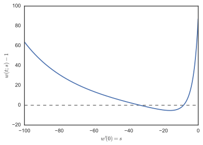
A boundary value problem is given as follows by Stoer and Burlisch[1] (Section 7.3.1).

w''(t)={\frac {3}{2}}w^{2},\quad w(0)=4,\quad w(1)=1

The initial value problem

w''(t)={\frac {3}{2}}w^{2},\quad w(0)=4,\quad w'(0)=s

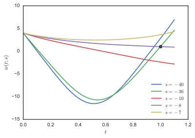
was solved for s = −1, −2, −3, ..., −100, and F(s) = w(1;s) − 1 plotted in the first figure. Inspecting the plot of F, we see that there are roots near −8 and −36. Some trajectories of w(t;s) are shown in the second figure.

Stoer and Burlisch[1] state that there are two solutions, which can be found by algebraic methods. These correspond to the initial conditions w′(0) = −8 and w′(0) = −35.9 (approximately).

The function F(s) = w(1;s) − 1.

Trajectories w(t;s) for s = w'(0) equal to −7, −8, −10, −36, and −40. The point (1,1) is marked with a circle.

Notes

Stoer, J. and Burlisch, R. Introduction to Numerical Analysis. New York: Springer-Verlag, 1980.

References

Press, WH; Teukolsky, SA; Vetterling, WT; Flannery, BP (2007). "Section 18.1. The Shooting Method". Numerical Recipes: The Art of Scientific Computing (3rd ed.). New York: Cambridge University Press. ISBN 978-0-521-88068-8.

External links

Brief Description of ODEPACK (at Netlib; contains LSODE)
Shooting method of solving boundary value problems – Notes, PPT, Maple, Mathcad, Matlab, Mathematica at Holistic Numerical Methods Institute

This article is issued from Wikipedia. The text is licensed under Creative Commons - Attribution - Sharealike. Additional terms may apply for the media files.

[Stoer1980-1] Stoer, J. and Burlisch, R. Introduction to Numerical Analysis. New York: Springer-Verlag, 1980.