Ordered dithering
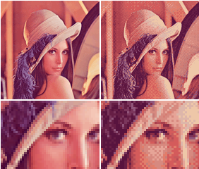
Ordered dithering is an image dithering algorithm. It is commonly used to display a continuous image on a display of smaller color depth. For example, Microsoft Windows uses it in 16-color graphics modes. The algorithm is characterized by noticeable crosshatch patterns in the result.
Threshold map
The algorithm reduces the number of colors by applying a threshold map M to the pixels displayed, causing some pixels to change color, depending on the distance of the original color from the available color entries in the reduced palette.
Threshold maps come in various sizes:
|
|


The map may be rotated or mirrored without affecting the effectiveness of the algorithm. This threshold map (for sides with length as power of two) is also known as an index matrix or Bayer matrix.[1]
Arbitrary size threshold maps can be devised with a simple rule: First fill each slot with a successive integers. Then reorder them such that the average distance between two successive numbers in the map is as large as possible, ensuring that the table "wraps" around at edges. For threshold maps whose dimensions are a power of two, the map can be generated recursively via:

The recursive expression can be calculated explicitly using only bit arithmetic:[2]
M(i, j) = bit_reverse(bit_interleave(bitwise_xor(i, j), i)) / n ^ 2
Pre-calculated threshold maps
Rather than storing map as a matrix of × integers from 0 to , depending on the exact hardware used to perform the dithering, it may be beneficial to pre-calculate the thresholds of the map. For this, the following formula can be used:


Mpre(i,j) = (Mint(i,j)+1) / n^2
This generates a standard threshold matrix.
for the 2×2 map:
|
|

this creates the pre-calculated map:
|
|

Additionally, the subtraction with 0.5 can be done during pre-processing as well:
Mpre(i,j) = (Mint(i,j)+1) / n^2 - 0.5
creating the pre-calculated map:
|
|

Yet another option is to instead change the range of color values to range 0— (for a ×). Note however that this operation has to happen once for every pixel, and should thus only be performed if storing the threshold map as integers (instead of floating point numbers) is crucial.
Algorithm
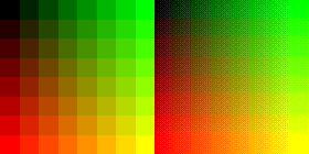
The ordered dithering algorithm renders the image normally, but for each pixel, it offsets its color value with a corresponding value from the threshold map according to its location, causing the pixel's value to be quantized to a different color if it exceeds the threshold.
For most dithering purposes, it is sufficient to simply add the threshold value to every pixel, or equivalently, to compare that pixel's value to the threshold: if the value of a pixel is less than the number in the corresponding cell of the matrix, plot that pixel black, otherwise, plot it white.
This slightly increases the average brightness of the image, and causes almost-white pixels to not be dithered. This is not a problem when using a gray scale palette (or any palette where the relative color distances are (nearly) constant), and it is often even desired, since the human eye perceives differences in darker colors more accurately than lighter ones, however, it produces incorrect results especially when using a small or arbitrary palette, so proper offsetting should be preferred.
The algorithm performs the following transformation on each color c of every pixel:

where M(i, j) is the threshold map on the i-th row and j-th column, c′ is the transformed color, and r is the amount of spread in color space. Assuming an RGB palette with 23N evenly chosen colors where each color (a triple of red, green and blue values) is represented by an octet from 0 to 255, one would typically choose:

The values read from the threshold map should preferably scale into the same range as the minimal difference between distinct colors in the target palette.
Because the algorithm operates on single pixels and has no conditional statements, it is very fast and suitable for real-time transformations. Additionally, because the location of the dithering patterns always stays the same relative to the display frame, it is less prone to jitter than error-diffusion methods, making it suitable for animations. Because the patterns are more repetitive than error-diffusion method, an image with ordered dithering compresses better. Ordered dithering is more suitable for line-art graphics as it will result in straighter lines and fewer anomalies.
The size of the map selected should be equal to or larger than the ratio of source colors to target colors. For example, when quantizing a 24 bpp image to 15 bpp (256 colors per channel to 32 colors per channel), the smallest map one would choose would be 4×2, for the ratio of 8 (256:32). This allows expressing each distinct tone of the input with different dithering patterns.
Notes
- Bayer, Bryce (June 11–13, 1973). "An optimum method for two-level rendition of continuous-tone pictures" (PDF). IEEE International Conference on Communications. 1: 11–15. Archived from the original (PDF) on 2013-05-12.
- Joel Yliluoma. “Arbitrary-palette positional dithering algorithm”
References
- Ordered Dithering (Graphics course project, Visgraf lab, Brazil)
- Dithering algorithms (Lee Daniel Crocker, Paul Boulay and Mike Morra)