Numerical differentiation

The simplest method is to use finite difference approximations.

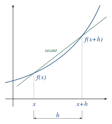
A simple two-point estimation is to compute the slope of a nearby secant line through the points (x, f(x)) and (x + h, f(x + h)).[1] Choosing a small number h, h represents a small change in x, and it can be either positive or negative. The slope of this line is

${\displaystyle {\frac {f(x+h)-f(x)}{h}}.}$

This expression is Newton's difference quotient (also known as a first-order divided difference).

The slope of this secant line differs from the slope of the tangent line by an amount that is approximately proportional to h. As h approaches zero, the slope of the secant line approaches the slope of the tangent line. Therefore, the true derivative of f at x is the limit of the value of the difference quotient as the secant lines get closer and closer to being a tangent line:

${\displaystyle f'(x)=\lim _{h\to 0}{\frac {f(x+h)-f(x)}{h}}.}$

Since immediately substituting 0 for h results in ${\displaystyle {\frac {0}{0}}}$ indeterminate form , calculating the derivative directly can be unintuitive.

Equivalently, the slope could be estimated by employing positions (x − h) and x.

Another two-point formula is to compute the slope of a nearby secant line through the points (x - h, f(x − h)) and (x + h, f(x + h)). The slope of this line is

${\displaystyle {\frac {f(x+h)-f(x-h)}{2h}}.}$

This formula is known as the symmetric difference quotient. In this case the first-order errors cancel, so the slope of these secant lines differ from the slope of the tangent line by an amount that is approximately proportional to ${\displaystyle h^{2}}$. Hence for small values of h this is a more accurate approximation to the tangent line than the one-sided estimation. However, although the slope is being computed at x, the value of the function at x is not involved.

The estimation error is given by

${\displaystyle R={\frac {-f^{(3)}(c)}{6}}h^{2}}$,

where ${\displaystyle c}$ is some point between ${\displaystyle x-h}$ and ${\displaystyle x+h}$. This error does not include the rounding error due to numbers being represented and calculations being performed in limited precision.

The symmetric difference quotient is employed as the method of approximating the derivative in a number of calculators, including TI-82, TI-83, TI-84, TI-85, all of which use this method with h = 0.001.[2][3]

Example showing the difficulty of choosing ${\displaystyle h}$ due to both rounding error and formula error

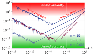
An important consideration in practice when the function is calculated using floating-point arithmetic is the choice of step size, h. If chosen too small, the subtraction will yield a large rounding error. In fact, all the finite-difference formulae are ill-conditioned[4] and due to cancellation will produce a value of zero if h is small enough.[5] If too large, the calculation of the slope of the secant line will be more accurately calculated, but the estimate of the slope of the tangent by using the secant could be worse.

For the numerical derivative formula evaluated at x and x + h, a choice for h that is small without producing a large rounding error is ${\displaystyle {\sqrt {\varepsilon }}x}$ (though not when x = 0), where the machine epsilon ε is typically of the order of 2.2×10⁻¹⁶.[6] A formula for h that balances the rounding error against the secant error for optimum accuracy is[7]

${\displaystyle h=2{\sqrt {\varepsilon \left|{\frac {f(x)}{f''(x)}}\right|}}}$

(though not when ${\displaystyle f''(x)=0}$), and to employ it will require knowledge of the function.

For single precision the problems are exacerbated because, although x may be a representable floating-point number, x + h almost certainly will not be. This means that x + h will be changed (by rounding or truncation) to a nearby machine-representable number, with the consequence that (x + h) − x will not equal h; the two function evaluations will not be exactly h apart. In this regard, since most decimal fractions are recurring sequences in binary (just as 1/3 is in decimal) a seemingly round step such as h = 0.1 will not be a round number in binary; it is 0.000110011001100...₂ A possible approach is as follows:

 h := sqrt(eps) * x;
 xph := x + h;
 dx := xph - x;
 slope := (F(xph) - F(x)) / dx;

However, with computers, compiler optimization facilities may fail to attend to the details of actual computer arithmetic and instead apply the axioms of mathematics to deduce that dx and h are the same. With C and similar languages, a directive that xph is a volatile variable will prevent this.

The classical finite-difference approximations for numerical differentiation are ill-conditioned. However, if ${\displaystyle f}$ is a holomorphic function, real-valued on the real line, which can be evaluated at points in the complex plane near ${\displaystyle x}$, then there are stable methods. For example,[5] the first derivative can be calculated by the complex-step derivative formula:[10][11][12]

${\displaystyle f^{\prime }(x)=\Im (f(x+\mathrm {i} h))/h+O(h^{2}),\quad \mathrm {i}$ :={\sqrt {-1}}.}

This formula can be obtained by Taylor series expansion:

${\displaystyle f(x+\mathrm {i} h)=f(x)+\mathrm {i} hf^{\prime }(x)-h^{2}f''(x)/2!-\mathrm {i} h^{3}f^{(3)}(x)/3!+\cdots .}$

The complex-step derivative formula is only valid for calculating first-order derivatives. A generalization of the above for calculating derivatives of any order employ multicomplex numbers, resulting in multicomplex derivatives.[13]

In general, derivatives of any order can be calculated using Cauchy's integral formula[14]:

${\displaystyle f^{(n)}(a)={\frac {n!}{2\pi i}}\oint _{\gamma }{\frac {f(z)}{(z-a)^{n+1}}}\,\mathrm {d} z,}$

where the integration is done numerically.

Using complex variables for numerical differentiation was started by Lyness and Moler in 1967.[15] A method based on numerical inversion of a complex Laplace transform was developed by Abate and Dubner.[16] An algorithm that can be used without requiring knowledge about the method or the character of the function was developed by Fornberg.[4]

Differential quadrature is the approximation of derivatives by using weighted sums of function values.[17][18] The name is in analogy with quadrature, meaning numerical integration, where weighted sums are used in methods such as Simpson's method or the Trapezoidal rule. There are various methods for determining the weight coefficients. Differential quadrature is used to solve partial differential equations.

• Automatic differentiation
• Five-point stencil
• Numerical integration
• Numerical ordinary differential equations
• Numerical smoothing and differentiation
• List of numerical analysis software

Wikibooks has a book on the topic of: Numerical Methods

• http://mathworld.wolfram.com/NumericalDifferentiation.html
• Numerical Differentiation Resources: Textbook notes, PPT, Worksheets, Audiovisual YouTube Lectures at Numerical Methods for STEM Undergraduate
• ftp://math.nist.gov/pub/repository/diff/src/DIFF Fortran code for the numerical differentiation of a function using Neville's process to extrapolate from a sequence of simple polynomial approximations.
• NAG Library numerical differentiation routines
• http://graphulator.com Online numerical graphing calculator with calculus function.
• Boost. Math numerical differentiation, including finite differencing and the complex step derivative
• Complex Step Differentiation
• Differentiation With(out) a Difference by Nicholas Higham, SIAM News.
• findiff Python project

References

- Richard L. Burden, J. Douglas Faires (2000), Numerical Analysis, (7th Ed), Brooks/Cole. ISBN 0-534-38216-9.
- Katherine Klippert Merseth (2003). Windows on Teaching Math: Cases of Middle and Secondary Classrooms. Teachers College Press. p. 34. ISBN 978-0-8077-4279-2.
- Tamara Lefcourt Ruby; James Sellers; Lisa Korf; Jeremy Van Horn; Mike Munn (2014). Kaplan AP Calculus AB & BC 2015. Kaplan Publishing. p. 299. ISBN 978-1-61865-686-5.
- Numerical Differentiation of Analytic Functions, B Fornberg – ACM Transactions on Mathematical Software (TOMS), 1981.
- Using Complex Variables to Estimate Derivatives of Real Functions, W. Squire, G. Trapp – SIAM REVIEW, 1998.
- Following Numerical Recipes in C, Chapter 5.7.
- p. 263.
- Abramowitz & Stegun, Table 25.2.
- Shilov, George. Elementary Real and Complex Analysis.
- Martins, J. R. R. A.; Sturdza, P.; Alonso, J. J. (2003). "The Complex-Step Derivative Approximation". ACM Transactions on Mathematical Software. 29 (3): 245–262. CiteSeerX 10.1.1.141.8002. doi:10.1145/838250.838251.