Lindhard theory

First, consider the long wavelength limit (${\displaystyle q\to 0}$).

For the denominator of the Lindhard formula, we get

${\displaystyle E_{k-q}-E_{k}={\frac {\hbar ^{2}}{2m}}(k^{2}-2{\vec {k}}\cdot {\vec {q}}+q^{2})-{\frac {\hbar ^{2}k^{2}}{2m}}\simeq -{\frac {\hbar ^{2}{\vec {k}}\cdot {\vec {q}}}{m}}}$,

and for the numerator of the Lindhard formula, we get

${\displaystyle f_{k-q}-f_{k}=f_{k}-{\vec {q}}\cdot \nabla _{k}f_{k}+\cdots -f_{k}\simeq -{\vec {q}}\cdot \nabla _{k}f_{k}}$.

Inserting these into the Lindhard formula and taking the ${\displaystyle \delta \to 0}$ limit, we obtain

${\displaystyle {\begin{alignedat}{2}\epsilon (0,\omega _{0})&\simeq 1+V_{q}\sum _{k,i}{\frac {q_{i}{\frac {\partial f_{k}}{\partial k_{i}}}}{\hbar \omega _{0}-{\frac {\hbar ^{2}{\vec {k}}\cdot {\vec {q}}}{m}}}}\\&\simeq 1+{\frac {V_{q}}{\hbar \omega _{0}}}\sum _{k,i}{q_{i}{\frac {\partial f_{k}}{\partial k_{i}}}}(1+{\frac {\hbar {\vec {k}}\cdot {\vec {q}}}{m\omega _{0}}})\\&\simeq 1+{\frac {V_{q}}{\hbar \omega _{0}}}\sum _{k,i}{q_{i}{\frac {\partial f_{k}}{\partial k_{i}}}}{\frac {\hbar {\vec {k}}\cdot {\vec {q}}}{m\omega _{0}}}\\&=1-V_{q}{\frac {q^{2}}{m\omega _{0}^{2}}}\sum _{k}{f_{k}}\\&=1-V_{q}{\frac {q^{2}N}{m\omega _{0}^{2}}}\\&=1-{\frac {4\pi e^{2}}{\epsilon q^{2}L^{3}}}{\frac {q^{2}N}{m\omega _{0}^{2}}}\\&=1-{\frac {\omega _{pl}^{2}}{\omega _{0}^{2}}}\end{alignedat}}}$,

where we used ${\displaystyle E_{k}=\hbar \omega _{k}}$, ${\displaystyle V_{q}={\frac {4\pi e^{2}}{\epsilon q^{2}L^{3}}}}$ and ${\displaystyle \omega _{pl}^{2}={\frac {4\pi e^{2}N}{\epsilon L^{3}m}}}$.

(In SI units, replace the factor ${\displaystyle 4\pi }$ by ${\displaystyle 1/\epsilon _{0}}$.)

This result is the same as the classical dielectric function.

Second, consider the static limit (${\displaystyle \omega +i\delta \to 0}$). The Lindhard formula becomes

${\displaystyle \epsilon (q,0)=1-V_{q}\sum _{k}{\frac {f_{k-q}-f_{k}}{E_{k-q}-E_{k}}}}$.

Inserting the above equalities for the denominator and numerator, we obtain

${\displaystyle \epsilon (q,0)=1-V_{q}\sum _{k,i}{\frac {-q_{i}{\frac {\partial f}{\partial k_{i}}}}{-{\frac {\hbar ^{2}{\vec {k}}\cdot {\vec {q}}}{m}}}}=1-V_{q}\sum _{k,i}{\frac {q_{i}{\frac {\partial f}{\partial k_{i}}}}{\frac {\hbar ^{2}{\vec {k}}\cdot {\vec {q}}}{m}}}}$.

Assuming a thermal equilibrium Fermi–Dirac carrier distribution, we get

${\displaystyle \sum _{i}{q_{i}{\frac {\partial f_{k}}{\partial k_{i}}}}=-\sum _{i}{q_{i}{\frac {\partial f_{k}}{\partial \mu }}{\frac {\partial \epsilon _{k}}{\partial k_{i}}}}=-\sum _{i}{q_{i}k_{i}{\frac {\hbar ^{2}}{m}}{\frac {\partial f_{k}}{\partial \mu }}}}$

here, we used ${\displaystyle \epsilon _{k}={\frac {\hbar ^{2}k^{2}}{2m}}}$ and ${\displaystyle {\frac {\partial \epsilon _{k}}{\partial k_{i}}}={\frac {\hbar ^{2}k_{i}}{m}}}$.

Therefore,

${\displaystyle {\begin{alignedat}{2}\epsilon (q,0)&=1+V_{q}\sum _{k,i}{\frac {q_{i}k_{i}{\frac {\hbar ^{2}}{m}}{\frac {\partial f_{k}}{\partial \mu }}}{\frac {\hbar ^{2}{\vec {k}}\cdot {\vec {q}}}{m}}}=1+V_{q}\sum _{k}{\frac {\partial f_{k}}{\partial \mu }}=1+{\frac {4\pi e^{2}}{\epsilon q^{2}}}{\frac {\partial }{\partial \mu }}{\frac {1}{L^{3}}}\sum _{k}{f_{k}}\\&=1+{\frac {4\pi e^{2}}{\epsilon q^{2}}}{\frac {\partial }{\partial \mu }}{\frac {N}{L^{3}}}=1+{\frac {4\pi e^{2}}{\epsilon q^{2}}}{\frac {\partial n}{\partial \mu }}\equiv 1+{\frac {\kappa ^{2}}{q^{2}}}.\end{alignedat}}}$

Here, ${\displaystyle \kappa }$ is the 3D screening wave number (3D inverse screening length) defined as ${\displaystyle \kappa ={\sqrt {{\frac {4\pi e^{2}}{\epsilon }}{\frac {\partial n}{\partial \mu }}}}}$.

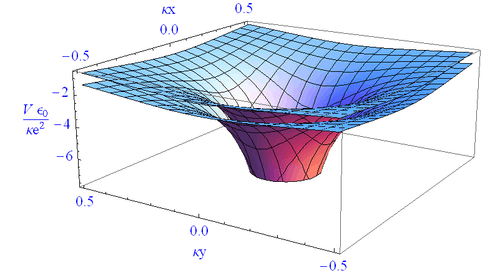
Then, the 3D statically screened Coulomb potential is given by

${\displaystyle V_{s}(q,\omega =0)\equiv {\frac {V_{q}}{\epsilon (q,\omega =0)}}={\frac {\frac {4\pi e^{2}}{\epsilon q^{2}L^{3}}}{\frac {q^{2}+\kappa ^{2}}{q^{2}}}}={\frac {4\pi e^{2}}{\epsilon L^{3}}}{\frac {1}{q^{2}+\kappa ^{2}}}}$.

And the Fourier transformation of this result gives

${\displaystyle V_{s}(r)=\sum _{q}{{\frac {4\pi e^{2}}{\epsilon L^{3}(q^{2}+\kappa ^{2})}}e^{i{\vec {q}}\cdot {\vec {r}}}}={\frac {e^{2}}{\epsilon r}}e^{-\kappa r}}$

known as the Yukawa potential. Note that in this Fourier transformation, which is basically a sum over all ${\displaystyle {\vec {q}}}$, we used the expression for small ${\displaystyle |{\vec {q}}|}$ for every value of ${\displaystyle {\vec {q}}}$ which is not correct.

Statically screened potential(upper curved surface) and Coulomb potential(lower curved surface) in three dimensions

For a degenerated Fermi gas (T=0), the Fermi energy is given by

${\displaystyle E_{\rm {F}}={\frac {\hbar ^{2}}{2m}}(3\pi ^{2}n)^{\frac {2}{3}}}$,

So the density is

${\displaystyle n={\frac {1}{3\pi ^{2}}}\left({\frac {2m}{\hbar ^{2}}}E_{\rm {F}}\right)^{\frac {3}{2}}}$.

At T=0, ${\displaystyle E_{\rm {F}}\equiv \mu }$, so ${\displaystyle {\frac {\partial n}{\partial \mu }}={\frac {3}{2}}{\frac {n}{E_{\rm {F}}}}}$.

Inserting this into the above 3D screening wave number equation, we obtain

${\displaystyle \kappa ={\sqrt {{\frac {4\pi e^{2}}{\epsilon }}{\frac {\partial n}{\partial \mu }}}}={\sqrt {\frac {6\pi e^{2}n}{\epsilon E_{\rm {F}}}}}}$.

This is the 3D Thomas–Fermi screening wave number.

For reference, Debye–Hückel screening describes the nondegenerate limit case. The result is ${\displaystyle \kappa ={\sqrt {\frac {4\pi e^{2}n\beta }{\epsilon }}}}$, the 3D Debye–Hückel screening wave number.

First, consider the long wavelength limit (${\displaystyle q\to 0}$).

For the denominator of the Lindhard formula,

${\displaystyle E_{k-q}-E_{k}={\frac {\hbar ^{2}}{2m}}(k^{2}-2{\vec {k}}\cdot {\vec {q}}+q^{2})-{\frac {\hbar ^{2}k^{2}}{2m}}\simeq -{\frac {\hbar ^{2}{\vec {k}}\cdot {\vec {q}}}{m}}}$,

and for the numerator,

${\displaystyle f_{k-q}-f_{k}=f_{k}-{\vec {q}}\cdot \nabla _{k}f_{k}+\cdots -f_{k}\simeq -{\vec {q}}\cdot \nabla _{k}f_{k}}$.

Inserting these into the Lindhard formula and taking the limit of ${\displaystyle \delta \to 0}$, we obtain

${\displaystyle {\begin{alignedat}{2}\epsilon (0,\omega )&\simeq 1+V_{q}\sum _{k,i}{\frac {q_{i}{\frac {\partial f_{k}}{\partial k_{i}}}}{\hbar \omega _{0}-{\frac {\hbar ^{2}{\vec {k}}\cdot {\vec {q}}}{m}}}}\\&\simeq 1+{\frac {V_{q}}{\hbar \omega _{0}}}\sum _{k,i}{q_{i}{\frac {\partial f_{k}}{\partial k_{i}}}}(1+{\frac {\hbar {\vec {k}}\cdot {\vec {q}}}{m\omega _{0}}})\\&\simeq 1+{\frac {V_{q}}{\hbar \omega _{0}}}\sum _{k,i}{q_{i}{\frac {\partial f_{k}}{\partial k_{i}}}}{\frac {\hbar {\vec {k}}\cdot {\vec {q}}}{m\omega _{0}}}\\&=1+{\frac {V_{q}}{\hbar \omega _{0}}}2\int d^{2}k({\frac {L}{2\pi }})^{2}\sum _{i,j}{q_{i}{\frac {\partial f_{k}}{\partial k_{i}}}}{\frac {\hbar k_{j}q_{j}}{m\omega _{0}}}\\&=1+{\frac {V_{q}L^{2}}{m\omega _{0}^{2}}}2\int {\frac {d^{2}k}{(2\pi )^{2}}}\sum _{i,j}{q_{i}q_{j}k_{j}{\frac {\partial f_{k}}{\partial k_{i}}}}\\&=1+{\frac {V_{q}L^{2}}{m\omega _{0}^{2}}}\sum _{i,j}{q_{i}q_{j}2\int {\frac {d^{2}k}{(2\pi )^{2}}}k_{j}{\frac {\partial f_{k}}{\partial k_{i}}}}\\&=1-{\frac {V_{q}L^{2}}{m\omega _{0}^{2}}}\sum _{i,j}{q_{i}q_{j}2\int {\frac {d^{2}k}{(2\pi )^{2}}}k_{k}{\frac {\partial f_{j}}{\partial k_{i}}}}\\&=1-{\frac {V_{q}L^{2}}{m\omega _{0}^{2}}}\sum _{i,j}{q_{i}q_{j}n\delta _{ij}}\\&=1-{\frac {2\pi e^{2}}{\epsilon qL^{2}}}{\frac {L^{2}}{m\omega _{0}^{2}}}q^{2}n\\&=1-{\frac {\omega _{pl}^{2}(q)}{\omega _{0}^{2}}},\end{alignedat}}}$

where we used ${\displaystyle E_{k}=\hbar \epsilon _{k}}$, ${\displaystyle V_{q}={\frac {2\pi e^{2}}{\epsilon qL^{2}}}}$ and ${\displaystyle \omega _{pl}^{2}(q)={\frac {2\pi e^{2}nq}{\epsilon m}}}$.

Second, consider the static limit (${\displaystyle \omega +i\delta \to 0}$). The Lindhard formula becomes

${\displaystyle \epsilon (q,0)=1-V_{q}\sum _{k}{\frac {f_{k-q}-f_{k}}{E_{k-q}-E_{k}}}}$.

Inserting the above equalities for the denominator and numerator, we obtain

${\displaystyle \epsilon (q,0)=1-V_{q}\sum _{k,i}{\frac {-q_{i}{\frac {\partial f}{\partial k_{i}}}}{-{\frac {\hbar ^{2}{\vec {k}}\cdot {\vec {q}}}{m}}}}=1-V_{q}\sum _{k,i}{\frac {q_{i}{\frac {\partial f}{\partial k_{i}}}}{\frac {\hbar ^{2}{\vec {k}}\cdot {\vec {q}}}{m}}}}$.

Assuming a thermal equilibrium Fermi–Dirac carrier distribution, we get

${\displaystyle \sum _{i}{q_{i}{\frac {\partial f_{k}}{\partial k_{i}}}}=-\sum _{i}{q_{i}{\frac {\partial f_{k}}{\partial \mu }}{\frac {\partial \epsilon _{k}}{\partial k_{i}}}}=-\sum _{i}{q_{i}k_{i}{\frac {\hbar ^{2}}{m}}{\frac {\partial f_{k}}{\partial \mu }}}}$

here, we used ${\displaystyle \epsilon _{k}={\frac {\hbar ^{2}k^{2}}{2m}}}$ and ${\displaystyle {\frac {\partial \epsilon _{k}}{\partial k_{i}}}={\frac {\hbar ^{2}k_{i}}{m}}}$.

Therefore,

${\displaystyle {\begin{alignedat}{2}\epsilon (q,0)&=1+V_{q}\sum _{k,i}{\frac {q_{i}k_{i}{\frac {\hbar ^{2}}{m}}{\frac {\partial f_{k}}{\partial \mu }}}{\frac {\hbar ^{2}{\vec {k}}\cdot {\vec {q}}}{m}}}=1+V_{q}\sum _{k}{\frac {\partial f_{k}}{\partial \mu }}=1+{\frac {2\pi e^{2}}{\epsilon qL^{2}}}{\frac {\partial }{\partial \mu }}\sum _{k}{f_{k}}\\&=1+{\frac {2\pi e^{2}}{\epsilon q}}{\frac {\partial }{\partial \mu }}{\frac {N}{L^{2}}}=1+{\frac {2\pi e^{2}}{\epsilon q}}{\frac {\partial n}{\partial \mu }}\equiv 1+{\frac {\kappa }{q}}.\end{alignedat}}}$

${\displaystyle \kappa }$ is 2D screening wave number(2D inverse screening length) defined as ${\displaystyle \kappa ={\frac {2\pi e^{2}}{\epsilon }}{\frac {\partial n}{\partial \mu }}}$.

Then, the 2D statically screened Coulomb potential is given by

${\displaystyle V_{s}(q,\omega =0)\equiv {\frac {V_{q}}{\epsilon (q,\omega =0)}}={\frac {2\pi e^{2}}{\epsilon qL^{2}}}{\frac {q}{q+\kappa }}={\frac {2\pi e^{2}}{\epsilon L^{2}}}{\frac {1}{q+\kappa }}}$.

It is known that the chemical potential of the 2-dimensional Fermi gas is given by

${\displaystyle \mu (n,T)={\frac {1}{\beta }}\ln {(e^{\hbar ^{2}\beta \pi n/m}-1)}}$,

and ${\displaystyle {\frac {\partial \mu }{\partial n}}={\frac {\hbar ^{2}\pi }{m}}{\frac {1}{1-e^{-\hbar ^{2}\beta \pi n/m}}}}$.

So, the 2D screening wave number is

${\displaystyle \kappa ={\frac {2\pi e^{2}}{\epsilon }}{\frac {\partial n}{\partial \mu }}={\frac {2\pi e^{2}}{\epsilon }}{\frac {m}{\hbar ^{2}\pi }}(1-e^{-\hbar ^{2}\beta \pi n/m})={\frac {2me^{2}}{\hbar ^{2}\epsilon }}f_{k=0}.}$

Note that this result is independent of n.

This time, consider some generalized case for lowering the dimension. The lower the dimension is, the weaker the screening effect. In lower dimension, some of the field lines pass through the barrier material wherein the screening has no effect. For the 1-dimensional case, we can guess that the screening affects only the field lines which are very close to the wire axis.

In real experiment, we should also take the 3D bulk screening effect into account even though we deal with 1D case like the single filament. The Thomas–Fermi screening has been applied to an electron gas confined to a filament and a coaxial cylinder.[5] For a K₂Pt(CN)₄Cl_0.32·2.6H₂0 filament, it was found that the potential within the region between the filament and cylinder varies as ${\displaystyle e^{-k_{\rm {eff}}r}/r}$ and its effective screening length is about 10 times that of metallic platinum.[5]

• Haug, Hartmut; W. Koch, Stephan (2004). Quantum Theory of the Optical and Electronic Properties of Semiconductors (4th ed.). World Scientific Publishing Co. Pte. Ltd. ISBN 978-981-238-609-0.

References

- Lindhard, Jens (1954). "On the properties of a gas of charged particles" (PDF). Danske Matematisk-fysiske Meddeleiser. 28 (8): 1–57. Retrieved 2016-09-28.
- N. W. Ashcroft and N. D. Mermin, Solid State Physics (Thomson Learning, Toronto, 1976)
- Andersen, Jens Ulrik; Sigmund, Peter (September 1998). "Jens Lindhard". Physics Today. 51 (9): 89–90. Bibcode:1998PhT....51i..89A. doi:10.1063/1.882460. ISSN 0031-9228.
- Smith, Henrik (1983). "The Lindhard Function and the Teaching of Solid State Physics". Physica Scripta. 28 (3): 287–293. Bibcode:1983PhyS...28..287S. doi:10.1088/0031-8949/28/3/005. ISSN 1402-4896.
- Davis, D. (1973). "Thomas-Fermi Screening in One Dimension". Physical Review B. 7 (1): 129–135. Bibcode:1973PhRvB...7..129D. doi:10.1103/PhysRevB.7.129.