Isoquant
An isoquant (derived from quantity and the Greek word iso, meaning equal), in microeconomics, is a contour line drawn through the set of points at which the same quantity of output is produced while changing the quantities of two or more inputs.[1][2] While an indifference curve mapping helps to solve the utility-maximizing problem of consumers, the isoquant mapping deals with the cost-minimization problem of producers. Isoquants are typically drawn along with isocost curves in capital-labor graphs, showing the technological tradeoff between capital and labor in the production function, and the decreasing marginal returns of both inputs. Adding one input while holding the other constant eventually leads to decreasing marginal output, and this is reflected in the shape of the isoquant. A family of isoquants can be represented by an isoquant map, a graph combining a number of isoquants, each representing a different quantity of output. Isoquants are also called equal product curves.
An isoquant shows that extent to which the firm in question has the ability to substitute between the two different inputs at will in order to produce the same level of output. An isoquant map can also indicate decreasing or increasing returns to scale based on increasing or decreasing distances between the isoquant pairs of fixed output increment, as output increases. If the distance between those isoquants increases as output increases, the firm's production function is exhibiting decreasing returns to scale; doubling both inputs will result in placement on an isoquant with less than double the output of the previous isoquant. Conversely, if the distance is decreasing as output increases, the firm is experiencing increasing returns to scale; doubling both inputs results in placement on an isoquant with more than twice the output of the original isoquant.
As with indifference curves, two isoquants can never cross. Also, every possible combination of inputs is on an isoquant. Finally, any combination of inputs above or to the right of an isoquant results in more output than any point on the isoquant. Although the marginal product of an input decreases as you increase the quantity of the input while holding all other inputs constant, the marginal product is never negative in the empirically observed range since a rational firm would never increase an input to decrease output.
An isoquants shows all those combinations of factors which produce same level of output. An isoquants is also known as equal product curve or iso-product curve. It describes the firm's alternative methods for producing a given level of output.
Shapes of Isoquants
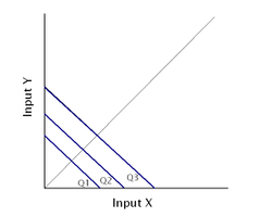
If the two inputs are perfect substitutes, the resulting isoquant map generated is represented in fig. A; with a given level of production Q3, input X can be replaced by input Y at an unchanging rate. The perfect substitute inputs do not experience decreasing marginal rates of return when they are substituted for each other in the production function.
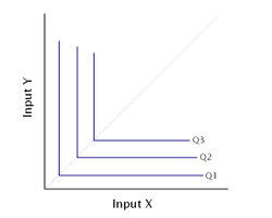
If the two inputs are perfect complements, the isoquant map takes the form of fig. B; with a level of production Q3, input X and input Y can only be combined efficiently in the certain ratio occurring at the kink in the isoquant. The firm will combine the two inputs in the required ratio to maximize profit.
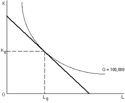
Isoquants are typically combined with isocost lines in order to solve a cost-minimization problem for given level of output. In the typical case shown in the top figure, with smoothly curved isoquants, a firm with fixed unit costs of the inputs will have isocost curves that are linear and downward sloped; any point of tangency between an isoquant and an isocost curve represents the cost-minimizing input combination for producing the output level associated with that isoquant. A line joining tangency points of isoquants and isocosts (with input prices held constant) is called the expansion path.[3]
Non convexity
Under the assumption of declining marginal rate of technical substitution, and hence a positive and finite elasticity of substitution, the isoquant is convex to the origin. A locally nonconvex isoquant can occur if there are sufficiently strong returns to scale in one of the inputs. In this case, there is a negative elasticity of substitution - as the ratio of input A to input B increases, the marginal product of A relative to B increases rather than decreases.
A nonconvex isoquant is prone to produce large and discontinous changes in the price minimizing input mix in response to price changes. Consider for example the case where the isoquant is globally nonconvex, and the isocost curve is linear. In this case the minimum cost mix of inputs will be a corner solution, and include only one input (for example either input A or input B). The choice of which input to use will depend on the relative prices. At some critical price ratio, the optimum input mix will shift from all input A to all input B and vice versa in response to a small change in relative prices.
See also
| Wikimedia Commons has media related to Isoquants. |
- Microeconomics
- Production, costs, and pricing
- Production theory basics
- Marginal rate of technical substitution
- Lerner diagram
References
- Varian, Hal R. (1992). Microeconomic Analysis (Third ed.). Norton. ISBN 0-393-95735-7.
- Chiang, Alpha C. (1984). Fundamental Methods of Mathematical Economics (Third ed.). McGraw-Hill. pp. 359–363. ISBN 0-07-010813-7.
- Salvatore, Dominick (1989). Schaum's outline of theory and problems of managerial economics, McGraw-Hill, ISBN 978-0-07-054513-7