Hypersimplex

In polyhedral combinatorics, a hypersimplex, Δ_d,k, is a convex polytope that generalizes the simplex. It is determined by two parameters d and k, and is defined as the convex hull of the d-dimensional vectors whose coefficients consist of k ones and d − k zeros. It forms a (d − 1)-dimensional polytope, because all of these vectors lie in a single (d − 1)-dimensional hyperplane.[1]

Standard hypersimplexes in R³
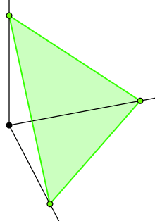
(3,1) Hyperplane: x + y + z = 1	(3,2) Hyperplane: x + y + z = 2

Properties

The number of vertices in Δ_d,k is ${\tbinom {d}{k}}$ .[1]

The graph formed by the vertices and edges of a hypersimplex Δ_d,k is the Johnson graph J(d,k).[2]

Alternative constructions

An alternative construction (for k ≤ d/2) is to take the convex hull of all (d − 1)-dimensional (0,1)-vectors that have either (k − 1) or k nonzero coordinates. This has the advantage of operating in a space that is the same dimension as the resulting polytope, but the disadavantage that the polytope it produces is less symmetric (although combinatorially equivalent to the result of the other construction).

A hypersimplex Δ_d,k is also the matroid polytope for a uniform matroid with d elements and rank k.[3]

Examples

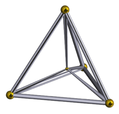
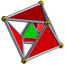
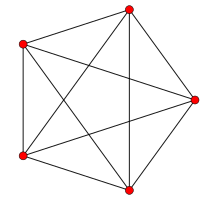
The hypersimplex with parameters (d,1) is a (d − 1)-simplex, with d vertices. The hypersimplex with parameters (4,2) is an octahedron, and the hypersimplex with parameters (5,2) is a rectified 5-cell.

Generally, every (k,d)-hypersimplex, Δ_d,k, corresponds to a uniform polytope, being the (k − 1)-rectified (d − 1)-simplex, with vertices positioned in the centers of all (k − 1)-face elements of a (d − 1)-simplex.

Examples (d = 3...6)
Name	Equilateral triangle	Tetrahedron (3-simplex)	Octahedron	5-cell (4-simplex)	Rectified 5-cell	5-simplex	Rectified 5-simplex	Birectified 5-simplex
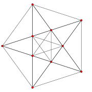
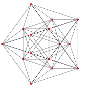
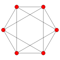
Δ_d,k = (d,k) = (d,d − k)	(3,1) (3,2)	(4,1) (4,3)	(4,2)	(5,1) (5,4)	(5,2) (5,3)	(6,1) (6,5)	(6,2) (6,4)	(6,3)
Vertices ${\tbinom {d}{k}}$	3	4	6	5	10	6	15	20
d-coordinates	(0,0,1) (0,1,1)	(0,0,0,1) (0,1,1,1)	(0,0,1,1)	(0,0,0,0,1) (0,1,1,1,1)	(0,0,0,1,1) (0,0,1,1,1)	(0,0,0,0,0,1) (0,1,1,1,1,1)	(0,0,0,0,1,1) (0,0,1,1,1,1)	(0,0,0,1,1,1)
Image
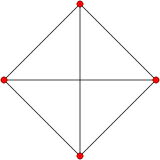
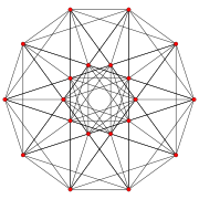
Graphs	J(3,1) = K₂	J(4,1) = K₃	J(4,2) = T(6,3)	J(5,1) = K₄	J(5,2)	J(6,1) = K₅	J(6,2)	J(6,3)
Coxeter diagrams
Schläfli symbols	{3} = r{3}	{3,3} = 2r{3,3}	r{3,3} = {3,4}	{3,3,3} = 3r{3,3,3}	r{3,3,3} = 2r{3,3,3}	{3,3,3,3} = 4r{3,3,3,3}	r{3,3,3,3} = 3r{3,3,3,3}	2r{3,3,3,3}
Facets	{ }	{3}		{3,3}	{3,3}, {3,4}	{3,3,3}	{3,3,3}, r{3,3,3}	r{3,3,3}

History

The hypersimplices were first studied and named in the computation of characteristic classes (an important topic in algebraic topology), by Gabrièlov, Gelʹfand & Losik (1975).[4][5]

References

Miller, Ezra; Reiner, Victor; Sturmfels, Bernd, Geometric Combinatorics, IAS/Park City mathematics series, 13, American Mathematical Society, p. 655, ISBN 9780821886953.
Rispoli, Fred J. (2008), The graph of the hypersimplex, arXiv:0811.2981, Bibcode:2008arXiv0811.2981R.
Grötschel, Martin (2004), "Cardinality homogeneous set systems, cycles in matroids, and associated polytopes", The Sharpest Cut: The Impact of Manfred Padberg and His Work, MPS/SIAM Ser. Optim., SIAM, Philadelphia, PA, pp. 99–120, MR 2077557. See in particular the remarks following Prop. 8.20 on p. 114.
Gabrièlov, A. M.; Gelʹfand, I. M.; Losik, M. V. (1975), "Combinatorial computation of characteristic classes. I, II", Akademija Nauk SSSR, 9 (2): 12–28, ibid. 9 (1975), no. 3, 5–26, MR 0410758.
Ziegler, Günter M. (1995), Lectures on Polytopes, Graduate Texts in Mathematics, 152, Springer-Verlag, New York, p. 20, doi:10.1007/978-1-4613-8431-1, ISBN 0-387-94365-X, MR 1311028.