Helmholtz equation

In mathematics, the eigenvalue problem for the laplace operator is called Helmholtz equation. It corresponds to the linear partial differential equation:

\nabla ^{2}f=-k^{2}f

Two sources of radiation in the plane, given mathematically by a function ƒ, which is zero in the blue region

The real part of the resulting field A, A is the solution to the inhomogeneous Helmholtz equation

(\nabla ^{2}-k^{2})A=-f

where $\nabla ^{2}$ is the Laplacian, $k$ is the eigenvalue (in the usual case of waves, it is called the wave number), and $f$ is the (eigen)function (in the usual case of waves, it simply represents the amplitude). It is used in a variety of cases of physics, including the wave equation and the diffusion equation, as well as in other sciences.

Motivation and uses

The Helmholtz equation often arises in the study of physical problems involving partial differential equations (PDEs) in both space and time. The Helmholtz equation, which represents a time-independent form of the wave equation, results from applying the technique of separation of variables to reduce the complexity of the analysis.

For example, consider the wave equation

\left(\nabla ^{2}-{\frac {1}{c^{2}}}{\frac {\partial ^{2}}{\partial t^{2}}}\right)u(\mathbf {r} ,t)=0.

Separation of variables begins by assuming that the wave function $u(\mathbf {r} ,t)$ is in fact separable:

u(\mathbf {r} ,t)=A(\mathbf {r} )T(t).

Substituting this form into the wave equation and then simplifying, we obtain the following equation:

{\frac {\nabla ^{2}A}{A}}={\frac {1}{c^{2}T}}{\frac {d^{2}T}{dt^{2}}}.

Notice that the expression on the left side depends only on $\mathbf {r}$ , whereas the right expression depends only on $t$ . As a result, this equation is valid in the general case if and only if both sides of the equation are equal to a constant value. This argument is key in the technique of solving linear partial differential equations by separation of variables. From this observation, we obtain two equations, one for $A(\mathbf {r} )$ , the other for $T(t)$ :

{\frac {\nabla ^{2}A}{A}}=-k^{2}

and

{\frac {1}{c^{2}T}}{\frac {d^{2}T}{dt^{2}}}=-k^{2},

where we have chosen, without loss of generality, the expression $-k^{2}$ for the value of the constant. (It is equally valid to use any constant $k$ as the separation constant; $-k^{2}$ is chosen only for convenience in the resulting solutions.)

Rearranging the first equation, we obtain the Helmholtz equation:

\nabla ^{2}A+k^{2}A=(\nabla ^{2}+k^{2})A=0.

Likewise, after making the substitution $\omega =kc$ , where $k$ is the wave number, and $\omega$ is the angular frequency, the second equation becomes

{\frac {d^{2}T}{dt^{2}}}+\omega ^{2}T=\left({\frac {d^{2}}{dt^{2}}}+\omega ^{2}\right)T=0,

We now have Helmholtz's equation for the spatial variable $\mathbf {r}$ and a second-order ordinary differential equation in time. The solution in time will be a linear combination of sine and cosine functions, whose exact form is determined by initial conditions, while the form of the solution in space will depend on the boundary conditions. Alternatively, integral transforms, such as the Laplace or Fourier transform, are often used to transform a hyperbolic PDE into a form of the Helmholtz equation.

Because of its relationship to the wave equation, the Helmholtz equation arises in problems in such areas of physics as the study of electromagnetic radiation, seismology, and acoustics.

Solving the Helmholtz equation using separation of variables

The solution to the spatial Helmholtz equation:

\nabla ^{2}A=-k^{2}A

can be obtained for simple geometries using separation of variables.

Vibrating membrane

The two-dimensional analogue of the vibrating string is the vibrating membrane, with the edges clamped to be motionless. The Helmholtz equation was solved for many basic shapes in the 19th century: the rectangular membrane by Siméon Denis Poisson in 1829, the equilateral triangle by Gabriel Lamé in 1852, and the circular membrane by Alfred Clebsch in 1862. The elliptical drumhead was studied by Émile Mathieu, leading to Mathieu's differential equation.

If the edges of a shape are straight line segments, then a solution is integrable or knowable in closed-form only if it is expressible as a finite linear combination of plane waves that satisfy the boundary conditions (zero at the boundary, i.e., membrane clamped).

If the domain is a circle of radius a, then it is appropriate to introduce polar coordinates r and θ. The Helmholtz equation takes the form

A_{rr}+{\frac {1}{r}}A_{r}+{\frac {1}{r^{2}}}A_{\theta \theta }+k^{2}A=0.

We may impose the boundary condition that A vanish if r = a; thus

A(a,\theta )=0.\,

The method of separation of variables leads to trial solutions of the form

A(r,\theta )=R(r)\Theta (\theta ),\,

where Θ must be periodic of period 2 $π$ . This leads to

\Theta ''+n^{2}\Theta =0,\,

and

r^{2}R''+rR'+r^{2}k^{2}R-n^{2}R=0.\,

It follows from the periodicity condition that

\Theta =\alpha \cos n\theta +\beta \sin n\theta ,\,

and that n must be an integer. The radial component R has the form

R(r)=\gamma J_{n}(\rho ),\,

where the Bessel function J_n(ρ) satisfies Bessel's equation

\rho ^{2}J_{n}''+\rho J_{n}'+(\rho ^{2}-n^{2})J_{n}=0,

and ρ = kr. The radial function J_n has infinitely many roots for each value of n, denoted by ρ_m,n. The boundary condition that A vanishes where r = a will be satisfied if the corresponding wavenumbers are given by

k_{m,n}={\frac {1}{a}}\rho _{m,n}.\,

The general solution A then takes the form of a generalized Fourier series of terms involving products of

\sin(n\theta ){\text{ or }}\cos(n\theta ),{\text{ and }}J_{n}(k_{m,n}r).

These solutions are the modes of vibration of a circular drumhead.

Three-dimensional solutions

In spherical coordinates, the solution is:

A(r,\theta ,\varphi )=\sum _{\ell =0}^{\infty }\sum _{m=-\ell }^{\ell }\left(a_{\ell m}j_{\ell }(kr)+b_{\ell m}y_{\ell }(kr)\right)Y_{\ell }^{m}(\theta ,\varphi ).

This solution arises from the spatial solution of the wave equation and diffusion equation. Here $j_{\ell }(kr)$ and $y_{\ell }(kr)$ are the spherical Bessel functions, and

Y_{\ell }^{m}(\theta ,\varphi )

are the spherical harmonics (Abramowitz and Stegun, 1964). Note that these forms are general solutions, and require boundary conditions to be specified to be used in any specific case. For infinite exterior domains, a radiation condition may also be required (Sommerfeld, 1949).

Writing $\mathbf {r_{0}} =(x,y,z)$ function $A(r_{0})$ has asymptotics

A(r_{0})={\frac {e^{ikr_{0}}}{r_{0}}}f\left({\frac {\mathbf {r} _{0}}{r_{0}}},k,u_{0}\right)+o\left({\frac {1}{r_{0}}}\right){\text{ as }}r_{0}\to \infty

where function f is called scattering amplitude and $u_{0}(r_{0})$ is the value of A at each boundary point $r_{0}$ .

Paraxial approximation

In the paraxial approximation of the Helmholtz equation,[1] the complex amplitude A is expressed as

A(\mathbf {r} )=u(\mathbf {r} )e^{ikz}

where u represents the complex-valued amplitude which modulates the sinusoidal plane wave represented by the exponential factor. Then under a suitable assumption, u approximately solves

\nabla _{\perp }^{2}u+2ik{\frac {\partial u}{\partial z}}=0,

where $\textstyle \nabla _{\perp }^{2}{\stackrel {\mathrm {def} }{=}}{\frac {\partial ^{2}}{\partial x^{2}}}+{\frac {\partial ^{2}}{\partial y^{2}}}$ is the transverse part of the Laplacian.

This equation has important applications in the science of optics, where it provides solutions that describe the propagation of electromagnetic waves (light) in the form of either paraboloidal waves or Gaussian beams. Most lasers emit beams that take this form.

The assumption under which the paraxial approximation is valid is that the z derivative of the amplitude function u is a slowly varying function of z:

{\bigg |}{\partial ^{2}u \over \partial z^{2}}{\bigg |}\ll {\bigg |}{k{\partial u \over \partial z}}{\bigg |}.

This condition is equivalent to saying that the angle θ between the wave vector k and the optical axis z is small: $\theta \ll 1$ .

The paraxial form of the Helmholtz equation is found by substituting the above-stated expression for the complex amplitude into the general form of the Helmholtz equation as follows:

\nabla ^{2}(u\left(x,y,z\right)e^{ikz})+k^{2}u\left(x,y,z\right)e^{ikz}=0.

Expansion and cancellation yields the following:

\left({\frac {\partial ^{2}}{\partial x^{2}}}+{\frac {\partial ^{2}}{\partial y^{2}}}\right)u(x,y,z)e^{ikz}+\left({\frac {\partial ^{2}}{\partial z^{2}}}u(x,y,z)\right)e^{ikz}+2\left({\frac {\partial }{\partial z}}u(x,y,z)\right)ik{e^{ikz}}=0.

Because of the paraxial inequality stated above, the ∂²u/∂z² term is neglected in comparison with the k·∂u/∂z term. This yields the paraxial Helmholtz equation. Substituting $u(\mathbf {r} )=A(\mathbf {r} )e^{-ikz}$ then gives the paraxial equation for the original complex amplitude A:

\nabla _{\perp }^{2}A+2ik{\frac {\partial A}{\partial z}}=0.

The Fresnel diffraction integral is an exact solution to the paraxial Helmholtz equation.[2]

There is even a subject named "Helmholtz optics" based on the equation, named in honour of Helmholtz. [3] [4] [5]

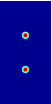
Inhomogeneous Helmholtz equation

The inhomogeneous Helmholtz equation is the equation

\nabla ^{2}A(x)+k^{2}A(x)=-f(x)\ {\text{ in }}\mathbb {R} ^{n},

where ƒ : Rⁿ → C is a function with compact support, and n = 1, 2, 3. This equation is very similar to the screened Poisson equation, and would be identical if the plus sign (in front of the k term) is switched to a minus sign.

In order to solve this equation uniquely, one needs to specify a boundary condition at infinity, which is typically the Sommerfeld radiation condition

\lim _{r\to \infty }r^{\frac {n-1}{2}}\left({\frac {\partial }{\partial r}}-ik\right)A(r{\hat {x}})=0

uniformly in ${\hat {x}}$ with $|{\hat {x}}|=1$ , where the vertical bars denote the Euclidean norm.

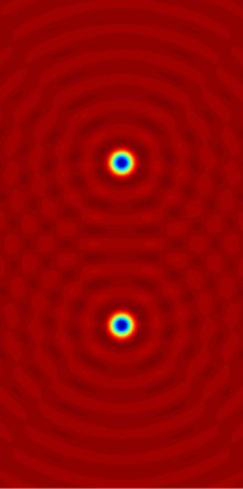
With this condition, the solution to the inhomogeneous Helmholtz equation is the convolution

A(x)=(G*f)(x)=\int \limits _{\mathbb {R} ^{n}}\!G(x-y)f(y)\,dy

(notice this integral is actually over a finite region, since $f$ has compact support). Here, $G$ is the Green's function of this equation, that is, the solution to the inhomogeneous Helmholtz equation with ƒ equaling the Dirac delta function, so G satisfies

\nabla ^{2}G(x)+k^{2}G(x)=-\delta (x){\text{ in }}\mathbb {R} ^{n}.\,

The expression for the Green's function depends on the dimension $n$ of the space. One has

G(x)={\frac {ie^{ik|x|}}{2k}}

for n = 1,

G(x)={\frac {i}{4}}H_{0}^{(1)}(k|x|)

for n = 2,[6] where $H_{0}^{(1)}$ is a Hankel function, and

G(x)={\frac {e^{ik|x|}}{4\pi |x|}}

for n = 3. Note that we have chosen the boundary condition that the Green's function is an outgoing wave for $|x|\to \infty$ .

Notes

J. W. Goodman. Introduction to Fourier Optics (2nd ed.). pp. 61–62.
Grella, R. (1982). "Fresnel propagation and diffraction and paraxial wave equation". Journal of Optics. 13 (6): 367–374. doi:10.1088/0150-536X/13/6/006.
Kurt Bernardo Wolf and Evgenii V. Kurmyshev, Squeezed states in Helmholtz optics, Physical Review A 47, 3365–3370 (1993).
Sameen Ahmed Khan, Wavelength-dependent modifications in Helmholtz Optics, International Journal of Theoretical Physics, 44(1), 95http://www.maa.org/programs/maa-awards/writing-awards/can-one-hear-the-shape-of-a-drum125 (January 2005).
Sameen Ahmed Khan, A Profile of Hermann von Helmholtz, Optics & Photonics News, Vol. 21, No. 7, pp. 7 (July/August 2010).
ftp://ftp.math.ucla.edu/pub/camreport/cam14-71.pdf

References

Abramowitz, Milton; Stegun, Irene, eds. (1964). Handbook of Mathematical functions with Formulas, Graphs and Mathematical Tables. New York: Dover Publications. ISBN 978-0-486-61272-0.

Riley, K. F.; Hobson, M. P.; Bence, S. J. (2002). "Chapter 19". Mathematical methods for physics and engineering. New York: Cambridge University Press. ISBN 978-0-521-89067-0.

Riley, K. F. (2002). "Chapter 16". Mathematical Methods for Scientists and Engineers. Sausalito, California: University Science Books. ISBN 978-1-891389-24-5.

Saleh, Bahaa E. A.; Teich, Malvin Carl (1991). "Chapter 3". Fundamentals of Photonics. Wiley Series in Pure and Applied Optics. New York: John Wiley & Sons. pp. 80–107. ISBN 978-0-471-83965-1.

Sommerfeld, Arnold (1949). "Chapter 16". Partial Differential Equations in Physics. New York: Academic Press. ISBN 978-0126546569.

Howe, M. S. (1998). Acoustics of fluid-structure interactions. New York: Cambridge University Press. ISBN 978-0-521-63320-8.

External links

Helmholtz Equation at EqWorld: The World of Mathematical Equations.
Hazewinkel, Michiel, ed. (2001) [1994], "Helmholtz equation", Encyclopedia of Mathematics, Springer Science+Business Media B.V. / Kluwer Academic Publishers, ISBN 978-1-55608-010-4
Vibrating Circular Membrane by Sam Blake, The Wolfram Demonstrations Project.
Green's functions for the wave, Helmholtz and Poisson equations in a two-dimensional boundless domain

This article is issued from Wikipedia. The text is licensed under Creative Commons - Attribution - Sharealike. Additional terms may apply for the media files.

[1] J. W. Goodman. Introduction to Fourier Optics (2nd ed.). pp. 61–62.

[2] Grella, R. (1982). "Fresnel propagation and diffraction and paraxial wave equation". Journal of Optics. 13 (6): 367–374. doi:10.1088/0150-536X/13/6/006.

[3] Kurt Bernardo Wolf and Evgenii V. Kurmyshev, Squeezed states in Helmholtz optics, Physical Review A 47, 3365–3370 (1993).

[4] Sameen Ahmed Khan, Wavelength-dependent modifications in Helmholtz Optics, International Journal of Theoretical Physics, 44(1), 95http://www.maa.org/programs/maa-awards/writing-awards/can-one-hear-the-shape-of-a-drum125 (January 2005).

[5] Sameen Ahmed Khan, A Profile of Hermann von Helmholtz, Optics & Photonics News, Vol. 21, No. 7, pp. 7 (July/August 2010).

[6] tp://ftp.math.ucla.edu/pub/camreport/cam14-71.pdf