Gillespie algorithm

A simple example may help to explain how the Gillespie algorithm works. Consider a system of molecules of two types: A and B. In the system A and B reversibly bind together to form AB dimers. So there are two reactions. The first is where one molecule of A reacts reversibly with one B molecule to form an AB dimer, and the second is where an AB dimer dissociates into an A and a B molecule. The reaction rate constant for a given single A molecule reacting with a given single B molecule is ${\displaystyle k_{\mathrm {D} }}$, and the reaction rate for an AB dimer breaking up is ${\displaystyle k_{\mathrm {B} }}$.

So, for example if at time t there is one molecule of each type then the rate of dimer formation is ${\displaystyle k_{\mathrm {D} }}$, while if there are ${\displaystyle n_{\mathrm {A} }}$ molecules of type A and ${\displaystyle n_{\mathrm {B} }}$ molecules of type B, the rate of dimer formation is ${\displaystyle k_{\mathrm {D} }n_{\mathrm {A} }n_{\mathrm {B} }}$. If there are ${\displaystyle n_{\mathrm {AB} }}$ dimers then the rate of dimer dissociation is ${\displaystyle k_{\mathrm {B} }n_{\mathrm {AB} }}$.

The total reaction rate, ${\displaystyle R_{\mathrm {TOT} }}$, at time t is then given by

${\displaystyle R_{\mathrm {TOT} }=k_{\mathrm {D} }n_{\mathrm {A} }n_{\mathrm {B} }+k_{\mathrm {B} }n_{\mathrm {AB} }}$

So, we have now described a simple model with two reactions. This definition is independent of the Gillespie algorithm. We will now describe how to apply the Gillespie algorithm to this system.

In the algorithm, we advance forward in time in two steps: calculating the time to the next reaction, and determining which of the possible reactions the next reaction is. Reactions are assumed to be completely random, so if the reaction rate at a time t is ${\displaystyle R_{\mathrm {TOT} }}$, then the time, δt, until the next reaction occurs is a random number drawn from exponential distribution function with mean ${\displaystyle 1/R_{\mathrm {TOT} }}$. Thus, we advance time from t to t + δt.

Plot of the number A molecules (black curve) and AB dimers as a function of time. As we started with 10 A and B molecules at time t=0, the number of B molecules is always equal to the number of A molecules and so it is not shown.

The probability that this reaction is an A molecule binding to a B molecule is simply the fraction of total rate due to this type of reaction, i.e.,

the probability that reaction is ${\displaystyle P({\ce {{A}+ B -> AB}})=k_{D}n_{A}n_{B}/R_{{\ce {TOT}}}}$

The probability that the next reaction is an AB dimer dissociating is just 1 minus that. So with these two probabilities we either form a dimer by reducing ${\displaystyle n_{\mathrm {A} }}$ and ${\displaystyle n_{\mathrm {B} }}$ by one, and increase ${\displaystyle n_{\mathrm {AB} }}$ by one, or we dissociate a dimer and increase ${\displaystyle n_{\mathrm {A} }}$ and ${\displaystyle n_{\mathrm {B} }}$ by one and decrease ${\displaystyle n_{\mathrm {AB} }}$ by one.

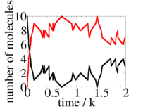
Now we have both advanced time to t + δt, and performed a single reaction. The Gillespie algorithm just repeats these two steps as many times as needed to simulate the system for however long we want (i.e., for as many reactions). The result of a Gillespie simulation that starts with ${\displaystyle n_{\mathrm {A} }=n_{\mathrm {B} }=10}$ and ${\displaystyle n_{\mathrm {AB} }=0}$ at t=0, and where ${\displaystyle k_{\mathrm {D} }=2}$ and ${\displaystyle k_{\mathrm {B} }=1}$, is shown at the right. For these parameter values, on average there are 8 ${\displaystyle n_{\mathrm {AB} }}$ dimers and 2 of A and B but due to the small numbers of molecules fluctuations around these values are large. The Gillespie algorithm is often used to study systems where these fluctuations are important.

That was just a simple example, with two reactions. More complex systems with more reactions are handled in the same way. All reaction rates must be calculated at each time step, and one chosen with probability equal to its fractional contribution to the rate. Time is then advanced as in this example.

The SIR model is a classic biological description of how certain diseases permeate through a fixed-size population. In its simplest form there are ${\displaystyle N}$ members of the population, whereby each member may be in one of three states -- susceptible, infected, or recovered -- at any instant in time, and each such member transitions irreversibly through these states according to the directed graph below. We can denote the number of susceptible members as ${\displaystyle n_{S}}$, the number of infected members as ${\displaystyle n_{I}}$, and the number of recovered members as ${\displaystyle n_{R}}$. Therefore we may also conclude that ${\displaystyle N=n_{S}+n_{I}+n_{R}}$ for any point in time.

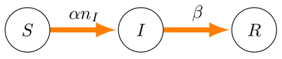
Further, a given susceptible member will transition to the infected state by coming into contact with any of the ${\displaystyle n_{I}}$ infected members, and so infection occurs with rate ${\displaystyle \alpha n_{I}}$ (dimensions of inverse time). A given member of the infected state recovers without dependence on any of the three states, which is specified by rate β (also with dimensions of inverse time). Given this basic scheme, it possible to construct the following non-linear system.

A single realization of the SIR epidemic as produced with an implementation of the Gillespie algorithm.

${\displaystyle {\frac {dn_{S}}{dt}}=-{\frac {\alpha n_{S}}{V}}n_{I}}$,

${\displaystyle {\frac {dn_{I}}{dt}}=\left({\frac {\alpha n_{S}}{V}}-\beta \right)n_{I}}$,

${\displaystyle {\frac {dn_{R}}{dt}}=\beta n_{I}}$.

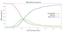
This system has no analytical solution. However, with the Gillespie algorithm, it can be simulated many times, and a regression technique such as least-squares may be applied to fit a polynomial over all of the trajectories. As the number of trajectories increases, such polynomial regression will asymptotically behave like an analytic solution. In addition to estimating the solution to an intractable problem like the SIR epidemic, the stochastic nature of each trajectory allows one to compute statistics other than ${\displaystyle \mathrm {E} [n|t]}$.

The trajectory presented in the above figure was simulated with the following Python implementation of the Gillespie algorithm.

import math
import random

# Input parameters ####################

# int; total population
N = 350

# float; maximum elapsed time
T = 100.0

# float; start time
t = 0.0

# float; spatial parameter
V = 100.0

# float; rate of infection after contact
_alpha = 10.0

# float; rate of cure
_beta = 0.5

# int; initial infected population
n_I = 1

#########################################

# Compute susceptible population, set recovered to zero
n_S = N - n_I
n_R = 0

# Initialize results list
SIR_data = []
SIR_data.append((t, n_S, n_I, n_R))

# Main loop
while t < T:
    if n_I == 0:
        break

    w1 = _alpha * n_S * n_I / V
    w2 = _beta * n_I
    W = w1 + w2

    dt = -math.log(random.uniform(0.0, 1.0)) / W
    t = t + dt

    if random.uniform(0.0, 1.0) < w1 / W:
        n_S = n_S - 1
        n_I = n_I + 1
    else:
        n_I = n_I - 1
        n_R = n_R + 1

    SIR_data.append((t, n_S, n_I, n_R))

with open('SIR_data.txt', 'w+') as fp:
    fp.write('\n'.join('%f %i %i %i' % x for x in SIR_data))