Gerchberg–Saxton algorithm
The Gerchberg–Saxton (GS) algorithm is an iterative algorithm for retrieving the phase of a pair of light distributions (or any other mathematically valid distribution) related via a propagating function, such as the Fourier transform, if their intensities at their respective optical planes are known.
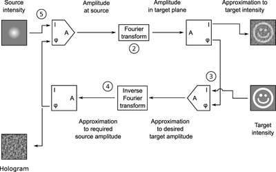

It is often necessary to know only the phase distribution from one of the planes, since the phase distribution on the other plane can be obtained by performing a Fourier transform on the plane whose phase is known. Although often used for two-dimensional signals, the GS algorithm is also valid for one-dimensional signals.
The paper by R. W. Gerchberg and W. O. Saxton on this algorithm is entitled “A practical algorithm for the determination of the phase from image and diffraction plane pictures,” and was published in Optik (35, 237–246 1972).
The pseudocode below performs the GS algorithm to obtain a phase distribution for the plane, Source, such that its Fourier transform would have the amplitude distribution of the plane, Target.
Pseudocode algorithm
Let:
 FT – forward Fourier transform
 IFT – inverse Fourier transform
 i – the imaginary unit, √−1 (square root of −1)
 exp – exponential function (exp(x) = ex)
 Target and Source be the Target and Source Amplitude planes respectively
 A, B, C & D be complex planes with the same dimension as Target and Source
 Amplitude – Amplitude-extracting function:
   e.g. for complex z = x + iy, amplitude(z) = sqrt(x·x + y·y)
       for real x, amplitude(x) = |x|
 Phase – Phase extracting function:
   e.g. Phase(z) = arctan(y / x)
end Let

algorithm Gerchberg–Saxton(Source, Target, Retrieved_Phase) is
    A := IFT(Target)
    while error criterion is not satisfied
        B := Amplitude(Source) × exp(i × Phase(A))
        C := FT(B)
        D := Amplitude(Target) × exp(i × Phase(C))
        A := IFT(D)
    end while
    Retrieved_Phase = Phase(A)
This is just one of the many ways to implement the GS algorithm. Aside from optimizations, others may start by performing a forward Fourier transform to the source distribution.
References
- R. W. Gerchberg and W. O. Saxton, "A practical algorithm for the determination of the phase from image and diffraction plane pictures,” Optik 35, 237 (1972)
- Press, WH; Teukolsky, SA; Vetterling, WT; Flannery, BP (2007). "Section 19.5.2. Deterministic Constraints: Projections onto Convex Sets". Numerical Recipes: The Art of Scientific Computing (3rd ed.). New York: Cambridge University Press. ISBN 978-0-521-88068-8.
External links
- Graphical explanatory material by Kevin Cowtan
- Dr W. Owen Saxton's pages ,
- Applications and publications on phase retrieval from the University of Rochester, Institute of Optics
- SLM ToolBox. A freeware Windows program for calculating holograms and displaying them on a spatial light modulator
- Graphical explanatory material by Kevin Cowtan
- A Python-Script of the GS by Dominik Doellerer