Denavit–Hartenberg parameters

A commonly used convention for selecting frames of reference in robotics applications is the Denavit and Hartenberg (D–H) convention which was introduced by Jacques Denavit and Richard S. Hartenberg. In this convention, coordinate frames are attached to the joints between two links such that one transformation is associated with the joint, [Z], and the second is associated with the link [X]. The coordinate transformations along a serial robot consisting of n links form the kinematics equations of the robot,

${\displaystyle [T]=[Z_{1}][X_{1}][Z_{2}][X_{2}]\ldots [X_{n-1}][Z_{n}][X_{n}],\!}$

where [T] is the transformation locating the end-link.

In order to determine the coordinate transformations [Z] and [X], the joints connecting the links are modeled as either hinged or sliding joints, each of which have a unique line S in space that forms the joint axis and define the relative movement of the two links. A typical serial robot is characterized by a sequence of six lines S_i, i = 1,...,6, one for each joint in the robot. For each sequence of lines S_i and S_i+1, there is a common normal line A_i,i+1. The system of six joint axes S_i and five common normal lines A_i,i+1 form the kinematic skeleton of the typical six degree of freedom serial robot. Denavit and Hartenberg introduced the convention that Z coordinate axes are assigned to the joint axes S_i and X coordinate axes are assigned to the common normals A_i,i+1.

This convention allows the definition of the movement of links around a common joint axis S_i by the screw displacement,

${\displaystyle [Z_{i}]={\begin{bmatrix}\cos \theta _{i}&-\sin \theta _{i}&0&0\\\sin \theta _{i}&\cos \theta _{i}&0&0\\0&0&1&d_{i}\\0&0&0&1\end{bmatrix}},}$

where θ_i is the rotation around and d_i is the slide along the Z axis—either of the parameters can be constants depending on the structure of the robot. Under this convention the dimensions of each link in the serial chain are defined by the screw displacement around the common normal A_i,i+1 from the joint S_i to S_i+1, which is given by

${\displaystyle [X_{i}]={\begin{bmatrix}1&0&0&r_{i,i+1}\\0&\cos \alpha _{i,i+1}&-\sin \alpha _{i,i+1}&0\\0&\sin \alpha _{i,i+1}&\cos \alpha _{i,i+1}&0\\0&0&0&1\end{bmatrix}},}$

where α_i,i+1 and r_i,i+1 define the physical dimensions of the link in terms of the angle measured around and distance measured along the X axis.

In summary, the reference frames are laid out as follows:

1. the ${\displaystyle z}$-axis is in the direction of the joint axis
2. the ${\displaystyle x}$-axis is parallel to the common normal: ${\displaystyle x_{n}=z_{n}\times z_{n-1}}$ (or away from zn-1)
   If there is no unique common normal (parallel ${\displaystyle z}$ axes), then ${\displaystyle d}$ (below) is a free parameter. The direction of ${\displaystyle x_{n}}$ is from ${\displaystyle z_{n-1}}$ to ${\displaystyle z_{n}}$, as shown in the video below.
3. the ${\displaystyle y}$-axis follows from the ${\displaystyle x}$- and ${\displaystyle z}$-axis by choosing it to be a right-handed coordinate system.

Four parameters

The four parameters of classic DH convention are shown in red text, which are ${\displaystyle \theta _{i},d_{i},a_{i},\alpha _{i}}$. With those four parameters, we can translate the coordinates from ${\displaystyle O_{i-1}X_{i-1}Y_{i-1}Z_{i-1}}$ to ${\displaystyle O_{i}X_{i}Y_{i}Z_{i}}$.

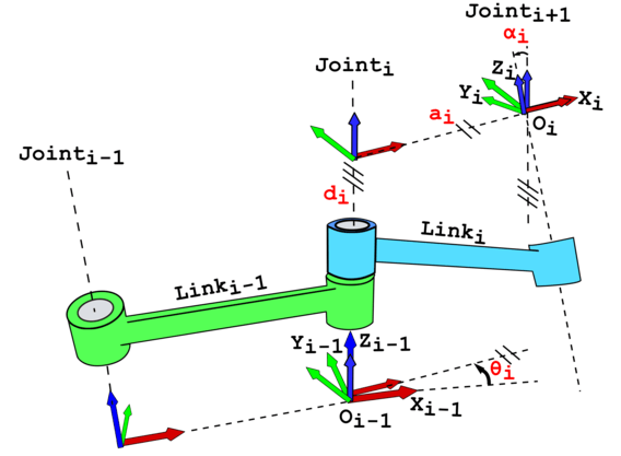
The following four transformation parameters are known as D–H parameters:.[4]

• ${\displaystyle d\,}$: offset along previous ${\displaystyle z}$ to the common normal
• ${\displaystyle \theta \,}$: angle about previous ${\displaystyle z}$, from old ${\displaystyle x}$ to new ${\displaystyle x}$
• ${\displaystyle r\,}$: length of the common normal (aka ${\displaystyle a}$, but if using this notation, do not confuse with ${\displaystyle \alpha }$). Assuming a revolute joint, this is the radius about previous ${\displaystyle z}$.
• ${\displaystyle \alpha \,}$: angle about common normal, from old ${\displaystyle z}$ axis to new ${\displaystyle z}$ axis

A visualization of D–H parameterization is available: YouTube

There is some choice in frame layout as to whether the previous ${\displaystyle x}$ axis or the next ${\displaystyle x}$ points along the common normal. The latter system allows branching chains more efficiently, as multiple frames can all point away from their common ancestor, but in the alternative layout the ancestor can only point toward one successor. Thus the commonly used notation places each down-chain ${\displaystyle x}$ axis collinear with the common normal, yielding the transformation calculations shown below.

We can note constraints on the relationships between the axes:

• the ${\displaystyle x_{n}}$-axis is perpendicular to both the ${\displaystyle z_{n-1}}$ and ${\displaystyle z_{n}}$ axes
• the ${\displaystyle x_{n}}$-axis intersects both ${\displaystyle z_{n-1}}$ and ${\displaystyle z_{n}}$ axes
• the origin of joint ${\displaystyle n}$ is at the intersection of ${\displaystyle x_{n}}$ and ${\displaystyle z_{n}}$
• ${\displaystyle y_{n}}$ completes a right-handed reference frame based on ${\displaystyle x_{n}}$ and ${\displaystyle z_{n}}$

It is common to separate a screw displacement into the product of a pure translation along a line and a pure rotation about the line,[5][6] so that

${\displaystyle [Z_{i}]=\operatorname {Trans} _{Z_{i}}(d_{i})\operatorname {Rot} _{Z_{i}}(\theta _{i}),}$

and

${\displaystyle [X_{i}]=\operatorname {Trans} _{X_{i}}(r_{i,i+1})\operatorname {Rot} _{X_{i}}(\alpha _{i,i+1}).}$

Using this notation, each link can be described by a coordinate transformation from the concurrent coordinate system to the previous coordinate system.

${\displaystyle {}^{n-1}T_{n}=\operatorname {Trans} _{z_{n-1}}(d_{n})\cdot \operatorname {Rot} _{z_{n-1}}(\theta _{n})\cdot \operatorname {Trans} _{x_{n}}(r_{n})\cdot \operatorname {Rot} _{x_{n}}(\alpha _{n})}$

Note that this is the product of two screw displacements, The matrices associated with these operations are:

${\displaystyle \operatorname {Trans} _{z_{n-1}}(d_{n})=\left[{\begin{array}{ccc|c}1&0&0&0\\0&1&0&0\\0&0&1&d_{n}\\\hline 0&0&0&1\end{array}}\right]}$

${\displaystyle \operatorname {Rot} _{z_{n-1}}(\theta _{n})=\left[{\begin{array}{ccc|c}\cos \theta _{n}&-\sin \theta _{n}&0&0\\\sin \theta _{n}&\cos \theta _{n}&0&0\\0&0&1&0\\\hline 0&0&0&1\end{array}}\right]}$

${\displaystyle \operatorname {Trans} _{x_{n}}(r_{n})=\left[{\begin{array}{ccc|c}1&0&0&r_{n}\\0&1&0&0\\0&0&1&0\\\hline 0&0&0&1\end{array}}\right]}$

${\displaystyle \operatorname {Rot} _{x_{n}}(\alpha _{n})=\left[{\begin{array}{ccc|c}1&0&0&0\\0&\cos \alpha _{n}&-\sin \alpha _{n}&0\\0&\sin \alpha _{n}&\cos \alpha _{n}&0\\\hline 0&0&0&1\end{array}}\right]}$

This gives:

${\displaystyle \operatorname {} ^{n-1}T_{n}=\left[{\begin{array}{ccc|c}\cos \theta _{n}&-\sin \theta _{n}\cos \alpha _{n}&\sin \theta _{n}\sin \alpha _{n}&r_{n}\cos \theta _{n}\\\sin \theta _{n}&\cos \theta _{n}\cos \alpha _{n}&-\cos \theta _{n}\sin \alpha _{n}&r_{n}\sin \theta _{n}\\0&\sin \alpha _{n}&\cos \alpha _{n}&d_{n}\\\hline 0&0&0&1\end{array}}\right]=\left[{\begin{array}{ccc|c}&&&\\&R&&T\\&&&\\\hline 0&0&0&1\end{array}}\right]}$

where R is the 3×3 submatrix describing rotation and T is the 3×1 submatrix describing translation.

In some books, the order of transformation for a pair of consecutive rotation and translation (such as ${\displaystyle d_{n}}$and ${\displaystyle \theta _{n}}$) is replaced. However, because matrix multiplication order for such pair does not matter, the result is the same. For example: ${\displaystyle \operatorname {Trans} _{z_{n-1}}(d_{n})\cdot \operatorname {Rot} _{z_{n-1}}(\theta _{n})=\operatorname {Rot} _{z_{n-1}}(\theta _{n})\cdot \operatorname {Trans} _{z_{n-1}}(d_{n})}$.

The Denavit and Hartenberg notation gives a standard methodology to write the kinematic equations of a manipulator. This is especially useful for serial manipulators where a matrix is used to represent the pose (position and orientation) of one body with respect to another.

The position of body ${\displaystyle n}$ with respect to ${\displaystyle n-1}$ may be represented by a position matrix indicated with the symbol ${\displaystyle T}$ or ${\displaystyle M}$

${\displaystyle \operatorname {} ^{n-1}T_{n}=M_{n-1,n}}$

This matrix is also used to transform a point from frame ${\displaystyle n}$ to ${\displaystyle n-1}$

${\displaystyle M_{n-1,n}=\left[{\begin{array}{ccc|c}R_{xx}&R_{xy}&R_{xz}&T_{x}\\R_{yx}&R_{yy}&R_{yz}&T_{y}\\R_{zx}&R_{zy}&R_{zz}&T_{z}\\\hline 0&0&0&1\end{array}}\right]}$

Where the upper left ${\displaystyle 3\times 3}$ submatrix of ${\displaystyle M}$ represents the relative orientation of the two bodies, and the upper right ${\displaystyle 3\times 1}$ represents their relative position or more specifically the body position in frame n − 1 represented with element of frame n.

The position of body ${\displaystyle k}$ with respect to body ${\displaystyle i}$ can be obtained as the product of the matrices representing the pose of ${\displaystyle j}$ with respect of ${\displaystyle i}$ and that of ${\displaystyle k}$ with respect of ${\displaystyle j}$

${\displaystyle M_{i,k}=M_{i,j}M_{j,k}}$

An important property of Denavit and Hartenberg matrices is that the inverse is

${\displaystyle M^{-1}=\left[{\begin{array}{ccc|c}&&&\\&R^{T}&&-R^{T}T\\&&&\\\hline 0&0&0&1\end{array}}\right]}$

where ${\displaystyle R^{T}}$ is both the transpose and the inverse of the orthogonal matrix ${\displaystyle R}$, i.e. ${\displaystyle R_{ij}^{-1}=R_{ij}^{T}=R_{ji}}$.

Further matrices can be defined to represent velocity and acceleration of bodies.[5][6] The velocity of body ${\displaystyle i}$ with respect to body ${\displaystyle j}$ can be represented in frame ${\displaystyle k}$ by the matrix

${\displaystyle W_{i,j(k)}=\left[{\begin{array}{ccc|c}0&-\omega _{z}&\omega _{y}&v_{x}\\\omega _{z}&0&-\omega _{x}&v_{y}\\-\omega _{y}&\omega _{x}&0&v_{z}\\\hline 0&0&0&0\end{array}}\right]}$

where ${\displaystyle \omega }$ is the angular velocity of body ${\displaystyle j}$ with respect to body ${\displaystyle i}$ and all the components are expressed in frame ${\displaystyle k}$; ${\displaystyle v}$ is the velocity of one point of body ${\displaystyle j}$ with respect to body ${\displaystyle i}$ (the pole). The pole is the point of ${\displaystyle j}$ passing through the origin of frame ${\displaystyle i}$.

The acceleration matrix can be defined as the sum of the time derivative of the velocity plus the velocity squared

${\displaystyle H_{i,j(k)}={\dot {W}}_{i,j(k)}+W_{i,j(k)}^{2}}$

The velocity and the acceleration in frame ${\displaystyle i}$ of a point of body ${\displaystyle j}$ can be evaluated as

${\displaystyle {\dot {P}}=W_{i,j}P}$

${\displaystyle {\ddot {P}}=H_{i,j}P}$

It is also possible to prove that

${\displaystyle {\dot {M}}_{i,j}=W_{i,j(i)}M_{i,j}}$

${\displaystyle {\ddot {M}}_{i,j}=H_{i,j(i)}M_{i,j}}$

Velocity and acceleration matrices add up according to the following rules

${\displaystyle W_{i,k}=W_{i,j}+W_{j,k}}$

${\displaystyle H_{i,k}=H_{i,j}+H_{j,k}+2W_{i,j}W_{j,k}}$

in other words the absolute velocity is the sum of the parent velocity plus the relative velocity; for the acceleration the Coriolis' term is also present.

The components of velocity and acceleration matrices are expressed in an arbitrary frame ${\displaystyle k}$ and transform from one frame to another by the following rule

${\displaystyle W_{(h)}=M_{h,k}W_{(k)}M_{k,h}}$

${\displaystyle H_{(h)}=M_{h,k}H_{(k)}M_{k,h}}$

For the dynamics three further matrices are necessary to describe the inertia ${\displaystyle J}$, the linear and angular momentum ${\displaystyle \Gamma }$, and the forces and torques ${\displaystyle \Phi }$ applied to a body.

Inertia ${\displaystyle J}$:

${\displaystyle J=\left[{\begin{array}{ccc|c}I_{xx}&I_{xy}&I_{xz}&x_{g}m\\I_{yx}&I_{yy}&I_{yz}&y_{g}m\\I_{zx}&I_{zy}&I_{zz}&z_{g}m\\\hline x_{g}m&y_{g}m&z_{g}m&m\end{array}}\right]}$

where ${\displaystyle m}$ is the mass, ${\displaystyle x_{g},\,y_{g},\,z_{g}}$ represent the position of the center of mass, and the terms ${\displaystyle I_{xx},\,I_{xy},\ldots }$ represent inertia and are defined as

${\displaystyle I_{xx}=\iint x^{2}\,dm}$

${\displaystyle {\begin{aligned}I_{xy}&=\iint xy\,dm\\I_{xz}&=\cdots \\&\,\,\,\vdots \end{aligned}}}$

Action matrix ${\displaystyle \Phi }$, containing force ${\displaystyle f}$ and torque ${\displaystyle t}$:

${\displaystyle \Phi =\left[{\begin{array}{ccc|c}0&-t_{z}&t_{y}&f_{x}\\t_{z}&0&-t_{x}&f_{y}\\-t_{y}&t_{x}&0&f_{z}\\\hline -f_{x}&-f_{y}&-f_{z}&0\end{array}}\right]}$

Momentum matrix ${\displaystyle \Gamma }$, containing linear ${\displaystyle \rho }$ and angular ${\displaystyle \gamma }$ momentum

${\displaystyle \Gamma =\left[{\begin{array}{ccc|c}0&-\gamma _{z}&\gamma _{y}&\rho _{x}\\\gamma _{z}&0&-\gamma _{x}&\rho _{y}\\-\gamma _{y}&\gamma _{x}&0&\rho _{z}\\\hline -\rho _{x}&-\rho _{y}&-\rho _{z}&0\end{array}}\right]}$

All the matrices are represented with the vector components in a certain frame ${\displaystyle k}$. Transformation of the components from frame ${\displaystyle k}$ to frame ${\displaystyle h}$ follows the rule

${\displaystyle {\begin{aligned}J_{(h)}&=M_{h,k}J_{(k)}M_{h,k}^{T}\\\Gamma _{(h)}&=M_{h,k}\Gamma _{(k)}M_{h,k}^{T}\\\Phi _{(h)}&=M_{h,k}\Phi _{(k)}M_{h,k}^{T}\end{aligned}}}$

The matrices described allow the writing of the dynamic equations in a concise way.

Newton's law:

${\displaystyle \Phi =HJ-JH^{t}\,}$

Momentum:

${\displaystyle \Gamma =WJ-JW^{t}\,}$

The first of these equations express the Newton's law and is the equivalent of the vector equation ${\displaystyle f=ma}$ (force equal mass times acceleration) plus ${\displaystyle t=J{\dot {\omega }}+\omega \times J\omega }$ (angular acceleration in function of inertia and angular velocity); the second equation permits the evaluation of the linear and angular momentum when velocity and inertia are known.

Some books such as Introduction to Robotics: Mechanics and Control (3rd Edition) [7] use modified DH parameters. The difference between the classic DH parameters and the modified DH parameters are the locations of the coordinates system attachment to the links and the order of the performed transformations.

Modified DH parameters

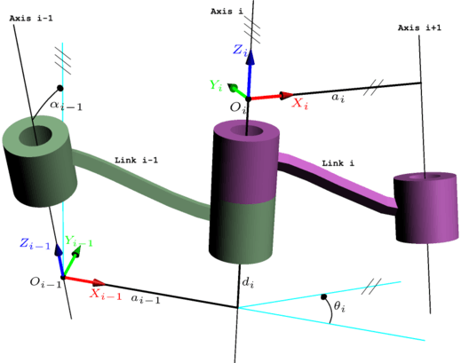
Compared with the classic DH parameters, the coordinates of frame ${\displaystyle O_{i-1}}$ is put on axis i − 1, not the axis i in classic DH convention. The coordinates of ${\displaystyle O_{i}}$ is put on the axis i, not the axis i + 1 in classic DH convention.

Another difference is that according to the modified convention, the transform matrix is given by the following order of operations:

${\displaystyle {}^{n-1}T_{n}=\operatorname {Rot} _{x_{n-1}}(\alpha _{n-1})\cdot \operatorname {Trans} _{x_{n-1}}(a_{n-1})\cdot \operatorname {Rot} _{z_{n}}(\theta _{n})\cdot \operatorname {Trans} _{z_{n}}(d_{n})}$

Thus, the matrix of the modified DH parameters becomes

${\displaystyle \operatorname {} ^{n-1}T_{n}=\left[{\begin{array}{ccc|c}\cos \theta _{n}&-\sin \theta _{n}&0&a_{n-1}\\\sin \theta _{n}\cos \alpha _{n-1}&\cos \theta _{n}\cos \alpha _{n-1}&-\sin \alpha _{n-1}&-d_{n}\sin \alpha _{n-1}\\\sin \theta _{n}\sin \alpha _{n-1}&\cos \theta _{n}\sin \alpha _{n-1}&\cos \alpha _{n-1}&d_{n}\cos \alpha _{n-1}\\\hline 0&0&0&1\end{array}}\right]}$

Note that some books (e.g.:[8]) use ${\displaystyle a_{n}}$ and ${\displaystyle \alpha _{n}}$ to indicate the length and twist of link n − 1 rather than link n. As a consequence, ${\displaystyle {}^{n-1}T_{n}}$ is formed only with parameters using the same subscript.

In some books, the order of transformation for a pair of consecutive rotation and translation (such as ${\displaystyle d_{n}}$and ${\displaystyle \theta _{n}}$) is replaced. However, because matrix multiplication order for such pair does not matter, the result is the same. For example: ${\displaystyle \operatorname {Trans} _{z_{n}}(d_{n})\cdot \operatorname {Rot} _{z_{n}}(\theta _{n})=\operatorname {Rot} _{z_{n}}(\theta _{n})\cdot \operatorname {Trans} _{z_{n}}(d_{n})}$.

Surveys of DH conventions and its differences have been published.[9][10] The visualization of the DH parameters definition can be easily observed and understood using the simulation software named RoboAnalyzer[11].

• Forward kinematics
• Inverse kinematics
• Kinematic chain
• Kinematics
• Robotics conventions
• Mechanical systems