Cronbach's alpha
Tau-equivalent reliability ()[1] is a single-administration test score reliability (i.e., the reliability of persons over items holding occasion fixed[2]) coefficient, commonly referred to as Cronbach's alpha or coefficient alpha. is the most famous and commonly used among reliability coefficients, but recent studies recommend not using it unconditionally.[3][4][5][6][7][8] Reliability coefficients based on structural equation modeling (SEM) are often recommended as its alternative.

Formula and calculation
Systematic and conventional formula
Let denote the observed score of item and denote the sum of all items in a test consisting of items. Let denote the covariance between and , denote the variance of , and denote the variance of . consists of item variances and inter-item covariances. That is, . Let denote the average of the inter-item covariances. That is, .


's "systematic"[1] formula is
.
The more frequently used but more difficult to understand version of the formula is
.


Calculation example
When applied to appropriate data
is applied to the following data that satisfies the condition of being tau-equivalent.


, ,


,

and .

When applied to inappropriate data
is applied to the following data that does not satisfy the condition of being tau-equivalent.


, ,

,

and .

Compare this value with the value of applying congeneric reliability to the same data.
Prerequisites for using tau-equivalent reliability
In order to use as a reliability coefficient, the data must satisfy the following conditions.
1) Unidimensionality
2) (Essential) tau-equivalence
3) Independence between errors
The conditions of being parallel, tau-equivalent, and congeneric
Parallel condition
At the population level, parallel data have equal inter-item covariances (i.e., non-diagonal elements of the covariance matrix) and equal variances (i.e., diagonal elements of the covariance matrix). For example, the following data satisfy the parallel condition. In parallel data, even if a correlation matrix is used instead of a covariance matrix, there is no loss of information. All parallel data are also tau-equivalent, but the reverse is not true. That is, among the three conditions, the parallel condition is most difficult to meet.
Tau-equivalent condition

At the population level, tau-equivalent data have equal covariances, but their variances may have different values. For example, the following data satisfies the condition of being tau-equivalent. All items in tau-equivalent data have equal discrimination or importance. All tau-equivalent data are also congeneric, but the reverse is not true.
Congeneric condition
At the population level, congeneric data need not have equal variances or covariances, provided they are unidimensional. For example, the following data meet the condition of being congeneric. All items in congeneric data can have different discrimination or importance.


Relationship with other reliability coefficients
Classification of single-administration reliability coefficients
Conventional names
There are numerous reliability coefficients. Among them, the conventional names of reliability coefficients that are related and frequently used are summarized as follows:[1]
| Split-half | Unidimensional | Multidimensional | |
|---|---|---|---|
| Parallel | Spearman-Brown formula | Standardized | (No conventional name) |
| Tau-equivalent | Flanagan formula Rulon formula Flanagan-Rulon formula Guttman's | Cronbach's coefficient Guttman's KR-20 Hoyt reliability | Stratified |
| Congeneric | Angoff-Feldt coefficient Raju(1970) coefficient | composite reliability construct reliability congeneric reliability coefficient unidimensional Raju(1977) coefficient | coefficient total MdDonald's multidimensional |


Combining row and column names gives the prerequisites for the corresponding reliability coefficient. For example, Cronbach's and Guttman's are reliability coefficients derived under the condition of being unidimensional and tau-equivalent.
Systematic names
Conventional names are disordered and unsystematic. Conventional names give no information about the nature of each coefficient, or give misleading information (e.g., composite reliability). Conventional names are inconsistent. Some are formulas, and others are coefficients. Some are named after the original developer, some are named after someone who is not the original developer, and others do not include the name of any person. While one formula is referred to by multiple names, multiple formulas are referred to by one notation (e.g., alphas and omegas). The proposed systematic names and their notation for these reliability coefficients are as follows: [1]
| Split-half | Unidimensional | Multidimensional | |
|---|---|---|---|
| Parallel | split-half parallel reliability() | parallel reliability() | multidimensional parallel reliability() |
| Tau-equivalent | split-half tau-equivalent reliability() | tau-equivalent reliability() | multidimensional tau-equivalent reliability() |
| Congeneric | split-half congeneric reliability () | congeneric reliability () | Bifactor model Bifactor reliability() Second-order factor model Second-order factor reliability() Correlated factor model Correlated factor reliability() |


Relationship with parallel reliability
is often referred to as coefficient alpha and is often referred to as standardized alpha. Because of the standardized modifier, is often mistaken for a more standard version than . There is no historical basis to refer to as standardized alpha. Cronbach (1951)[9] did not refer to this coefficient as alpha, nor did it recommend using it. was rarely used before the 1970s. As SPSS began to provide under the name of standardized alpha, this coefficient began to be used occasionally [10]. The use of is not recommended because the parallel condition is difficult to meet in real-world data.
Relationship with split-half tau-equivalent reliability
equals the average of the values obtained for all possible split-halves. This relationship, proved by Cronbach (1951)[9], is often used to explain the intuitive meaning of . However, this interpretation overlooks the fact that underestimes reliability when applied to data that are not tau-equivalent. At the population level, the maximum of all possible values is closer to reliability than the average of all possible values.[6] This mathematical fact was already known even before the publication of Cronbach (1951).[11] A comparative study[12] reports that the maximum of is the most accurate reliability coefficient.
Revelle (1979)[13] refers to the minimum of all possible values as coefficient , and recommends that provides complementary information that does not.[5]

Relationship with congeneric reliability
If the assumptions of unidimensionality and tau-equivalence are satisfied, equals .
If unidimensionality is satisfied but tau-equivalence is not satisfied, is smaller than [6].
is the most commonly used reliability coefficient after . Users tend to present both, rather than replacing with [1].
A study investigating studies that presented both coefficients reports that is .02 smaller than on average.[14]
Relationship with multidimensional reliability coefficients and

If is applied to multidimensional data, its value is smaller than multidimensional reliability coefficients and larger than .[1]
Relationship with Intraclass correlation
is said to be equal to the stepped-up consistency version of the intraclass correlation coefficient, which is commonly used in observational studies. But this is only conditionally true. In terms of variance components, this condition is, for item sampling: if and only if the value of the item (rater, in the case of rating) variance component equals zero. If this variance component is negative, will underestimate the stepped-up intra-class correlation coefficient; if this variance component is positive, will overestimate this stepped-up intra-class correlation coefficient.
History[10]
Before 1937
[15][16] was the only known reliability coefficient. The problem was that the reliability estimates depended on how the items were split in half (e.g., odd/even or front/back). Criticism was raised against this unreliability, but for more than 20 years no fundamental solution was found.[17]
Kuder and Richardson (1937)
Kuder and Richardson (1937)[18] developed several reliability coefficients that could overcome the problem of . They did not give the reliability coefficients particular names. Equation 20 in their article is . This formula is often referred to as Kuder-Richardson Formula 20, or KR-20. They dealt with cases where the observed scores were dichotomous (e.g., correct or incorrect), so the expression of KR-20 is slightly different from the conventional formula of . A review of this paper reveals that they did not present a general formula because they did not need to, not because they were not able to. Let denote the correct answer ratio of item , and denote the incorrect answer ratio of item (). The formula of KR-20 is as follows.


Since , KR-20 and have the same meaning.

Between 1937 and 1951
Several studies published the general formula of KR-20
Kuder and Richardson (1937) made unnecessary assumptions to derive . Several studies have derived in a different way from Kuder and Richardson (1937).
Hoyt (1941)[19] derived using ANOVA (Analysis of variance). Cyril Hoyt may be considered the first developer of the general formula of the KR-20, but he did not explicitly present the formula of .
The first expression of the modern formula of appears in Jackson and Ferguson (1941)[20]. The version they presented is as follows. Edgerton and Thompson (1942)[21] used the same version.

Guttman (1945)[11] derived six reliability formulas, each denoted by . Louis Guttman proved that all of these formulas were always less than or equal to reliability, and based on these characteristics, he referred to these formulas as 'lower bounds of reliability'. Guttman's is , and is . He proved that is always greater than or equal to (i.e., more accurate). At that time, all calculations were done with paper and pencil, and since the formula of was simpler to calculate, he mentioned that was useful under certain conditions.


Gulliksen (1950)[22] derived with fewer assumptions than previous studies. The assumption he used is essential tau-equivalence in modern terms.
Recognition of KR-20's original formula and general formula at the time
The two formulas were recognized to be exactly identical, and the expression of general formula of KR-20 was not used. Hoyt[19] explained that his method "gives precisely the same result" as KR-20 (p.156). Jackson and Ferguson[20] stated that the two formulas are "identical"(p.74). Guttman[11] said is "algebraically identical" to KR-20 (p.275). Gulliksen[22] also admitted that the two formulas are “identical”(p.224).
Even studies critical of KR-20 did not point out that the original formula of KR-20 could only be applied to dichotomous data.[23]
Criticism of underestimation of KR-20
Developers[18] of this formula reported that consistently underestimates reliability. Hoyt[24] argued that this characteristic alone made more recommendable than the traditional split-half technique, which was unknown whether to underestimate or overestimate reliability.
Cronbach (1943)[23] was critical of the underestimation of . He was concerned that it was not known how much underestimated reliability. He criticized that the underestimation was likely to be excessively severe, such that could sometimes lead to negative values. Because of these problems, he argued that could not be recommended as an alternative to the split-half technique.
Cronbach (1951)
As with previous studies[19][11][20][22], Cronbach (1951)[9] invented another method to derive . His interpretation was more intuitively attractive than those of previous studies. That is, he proved that equals the average of values obtained for all possible split-halves. He criticized that the name KR-20 was weird and suggested a new name, coefficient alpha. His approach has been a huge success. However, he not only omitted some key facts, but also gave an incorrect explanation.
First, he positioned coefficient alpha as a general formula of KR-20, but omitted the explanation that existing studies had published the precisely identical formula. Those who read only Cronbach (1951) without background knowledge could misunderstand that he was the first to develop the general formula of KR-20.
Second, he did not explain under what condition equals reliability. Non-experts could misunderstand that was a general reliability coefficient that could be used for all data regardless of prerequisites.
Third, he did not explain why he changed his attitude toward . In particular, he did not provide a clear answer to the underestimation problem of , which he himself[23] had criticized.
Fourth, he argued that a high value of indicated homogeneity of the data.
After 1951
Novick and Lewis (1967)[25] proved the necessary and sufficient condition for to be equal to reliability, and named it the condition of being essentially tau-equivalent.
Cronbach (1978)[2] mentioned that the reason Cronbach (1951) received a lot of citations was "mostly because [he] put a brand name on a common-place coefficient"(p.263)[1]. He explained that he had originally planned to name other types of reliability coefficients (e.g., inter-rater reliability or test-retest reliability) in consecutive Greek letter (e.g., , , ), but later changed his mind.


Cronbach and Schavelson (2004)[26] encouraged readers to use generalizability theory rather than . He opposed the use of the name Cronbach's alpha. He explicitly denied the existence of existing studies that had published the general formula of KR-20 prior to Cronbach (1951).
Common misconceptions about tau-equivalent reliability[6]
The value of tau-equivalent reliability ranges between zero and one
By definition, reliability cannot be less than zero and cannot be greater than one. Many textbooks mistakenly equate with reliability and give an inaccurate explanation of its range. can be less than reliability when applied to data that are not tau-equivalent. Suppose that copied the value of as it is, and copied by multiplying the value of by -1. The covariance matrix between items is as follows, .


Negative can occur for reasons such as negative discrimination or mistakes in processing reversely scored items.
Unlike , SEM-based reliability coefficients (e.g., ) are always greater than or equal to zero.
This anomaly was first pointed out by Cronbach (1943)[23] to criticize , but Cronbach (1951)[9] did not comment on this problem in his article, which discussed all conceivable issues related and he himself[26] described as being "encyclopedic" (p.396).
If there is no measurement error, the value of tau-equivalent reliability is one
This anomaly also originates from the fact that underestimates reliability. Suppose that copied the value of as it is, and copied by multiplying the value of by two. The covariance matrix between items is as follows, .

For the above data, both and have a value of one.
The above example is presented by Cho and Kim (2015)[6].
A high value of tau-equivalent reliability indicates homogeneity between the items
Many textbooks refer to as an indicator of homogeneity between items. This misconception stems from the inaccurate explanation of Cronbach (1951)[9] that high values show homogeneity between the items. Homogeneity is a term that is rarely used in the modern literature, and related studies interpret the term as referring to unidimensionality. Several studies have provided proofs or counterexamples that high values do not indicate unidimensionality.[27][6][28][29][30][31]See counterexamples below.


in the unidimensional data above.

in the multidimensional data above.
The above data have , but are multidimensional.

The above data have , but are unidimensional.

Unidimensionality is a prerequisite for . You should check unidimensionality before calculating , rather than calculating to check unidimensionality.[1]
A high value of tau-equivalent reliability indicates internal consistency
The term internal consistency is commonly used in the reliability literature, but its meaning is not clearly defined. The term is sometimes used to refer to a certain kind of reliability (e.g., internal consistency reliability), but it is unclear exactly which reliability coefficients are included here, in addition to . Cronbach (1951)[9] used the term in several senses without an explicit definition. Cho and Kim (2015)[6] showed that is not an indicator of any of these.
Removing items using "alpha if item deleted" always increases reliability
Removing an item using "alpha if item deleted" may result in 'alpha inflation,' where sample-level reliability is reported to be higher than population-level reliability.[32] It may also reduces population-level reliability.[33] The elimination of less-reliable items should be based not only on a statistical basis, but also on a theoretical and logical basis. It is also recommended that the whole sample be divided into two and cross-validated.[32]
Ideal reliability level and how to increase reliability
Nunnally's recommendations for the level of reliability
The most frequently cited source of how much reliability coefficients should be is Nunnally's book.[34][35][36] However, his recommendations are cited contrary to his intentions. What he meant was to apply different criteria depending on the purpose or stage of the study. However, regardless of the nature of the research, such as exploratory research, applied research, and scale development research, a criterion of .7 is universally used.[37] .7 is the criterion he recommended for the early stages of a study, which most studies published in the journal are not. Rather than .7, the criterion of .8 referred to applied research by Nunnally is more appropriate for most empirical studies.[37]
| 1st edition[34] | 2nd[35] & 3rd[36] edition | |
|---|---|---|
| Early stage of research | .5 or .6 | .7 |
| Applied research | .8 | .8 |
| When making important decisions | .95 (minimum .9) | .95 (minimum .9) |
His recommendation level did not imply a cutoff point. If a criterion means a cutoff point, it is important whether or not it is met, but it is unimportant how much it is over or under. He did not mean that it should be strictly .8 when referring to the criteria of .8. If the reliability has a value near .8 (e.g., 78), it can be considered that his recommendation has been met.[38]
His idea was that there is a cost to increasing reliability, so there is no need to try to obtain maximum reliability in every situation.
Cost to obtain a high level of reliability
Many textbooks explain that the higher the value of reliability, the better. The potential side effects of high reliability are rarely discussed. However, the principle of sacrificing something to get one also applies to reliability.
Trade-off between reliability and validity[6]
Measurements with perfect reliability lack validity. For example, a person who take the test with the reliability of one will get a perfect score or a zero score, because the examinee who give the correct answer or incorrect answer on one item will give the correct answer or incorrect answer on all other items. The phenomenon in which validity is sacrificed to increase reliability is called attenuation paradox.[39][40]
A high value of reliability can be in conflict with content validity. For high content validity, each item should be constructed to be able to comprehensively represent the content to be measured. However, a strategy of repeatedly measuring essentially the same question in different ways is often used only for the purpose of increasing reliability.[41][42].
Trade-off between reliability and efficiency
When the other conditions are equal, reliability increases as the number of items increases. However, the increase in the number of items hinders the efficiency of measurements.
Methods to increase reliability
Despite the costs associated with increasing reliability discussed above, a high level of reliability may be required. The following methods can be considered to increase reliability.
Before data collection
Eliminate the ambiguity of the measurement item.
Do not measure what the respondents do not know.
Increase the number of items. However, care should be taken not to excessively inhibit the efficiency of the measurement.
Use a scale that is known to be highly reliable.[43]
Conduct a pretest. Discover in advance the problem of reliability.
Exclude or modify items that are different in content or form from other items (e.g., reversely scored items).
After data collection
Remove the problematic items using "alpha if item deleted". However, this deletion should be accompanied by a theoretical rationale.
Use a more accurate reliability coefficient than . For example, is .02 larger than on average.[14]
Which reliability coefficient to use
Should we continue to use tau-equivalent reliability?
is used in an overwhelming proportion. A study estimates that approximately 97% of studies use as a reliability coefficient[1].
However, simulation studies comparing the accuracy of several reliability coefficients have led to the common result that is an inaccurate reliability coefficient.[44][12][5][45][46]
Methodological studies are critical of the use of . Simplifying and classifying the conclusions of existing studies are as follows.
(1) Conditional use: Use only when certain conditions are met.[1][6][8]
(2) Opposition to use: is inferior and should not be used. [47][4][48][5][3][49]
Alternatives to tau-equivalent reliability
Existing studies are practically unanimous in that they oppose the widespread practice of using unconditionally for all data. However, different opinions are given on which reliability coefficient should be used instead of .
Different reliability coefficients ranked first in each simulation study[44][12][5][45][46] comparing the accuracy of several reliability coefficients.[6]
The majority opinion is to use SEM-based reliability coefficients as an alternative to .[1][6][47][4][48][8][5][49]
However, there is no consensus on which of the several SEM-based reliability coefficients (e.g., unidimensional or multidimensional models) is the best to use.
Some people say [5] as an alternative, but shows information that is completely different from reliability. is a type of coefficient comparable to Revelle's .[13][5] They do not substitute, but complement reliability.[1]

Among SEM-based reliability coefficients, multidimensional reliability coefficients are rarely used, and the most commonly used is .[1]

Software for SEM-based reliability coefficients
General-purpose statistical software such as SPSS and SAS include a function to calculate . Users who don't know the formula of have no problem in obtaining the estimates with just a few mouse clicks.
SEM software such as AMOS, LISREL, and MPLUS does not have a function to calculate SEM-based reliability coefficients. Users need to calculate the result by inputting it to the formula. To avoid this inconvenience and possible error, even studies reporting the use of SEM rely on instead of SEM-based reliability coefficients.[1] There are a few alternatives to automatically calculate SEM-based reliability coefficients.
1) R (free): The psych package [50] calculates various reliability coefficients.
2) EQS (paid)[51]: This SEM software has a function to calculate reliability coefficients.
3) RelCalc (free)[1]: Available with Microsoft Excel. can be obtained without the need for SEM software. Various multidimensional SEM reliability coefficients and various types of can be calculated based on the results of SEM software.
Derivation of formula[1]
Assumption 1. The observed score of an item consists of the true score of the item and the error of the item, which is independent of the true score.

Lemma.

Assumption 2. Errors are independent of each other.

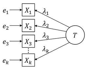
Assumption 3. (The assumption of being essentially tau-equivalent) The true score of an item consists of the true score common to all items and the constant of the item.

Let denote the sum of the item true scores.


The variance of is called the true score variance.
Definition. Reliability is the ratio of true score variance to observed score variance.

The following relationship is established from the above assumptions.


Therefore, the covariance matrix between items is as follows.


You can see that equals the mean of the covariances between items. That is,


Let denote the reliability when satisfying the above assumptions. is:
References
- Cho, E. (2016). Making reliability reliable: A systematic approach to reliability coefficients. Organizational Research Methods, 19(4), 651–682. https://doi.org/10.1177/1094428116656239
- Cronbach, L. J. (1978). Citation classics. Current Contents, 13, 263.
- Sijtsma, K. (2009). On the use, the misuse, and the very limited usefulness of Cronbach’s alpha. Psychometrika, 74(1), 107–120. https://doi.org/10.1007/s11336-008-9101-0
- Green, S. B., & Yang, Y. (2009). Commentary on coefficient alpha: A cautionary tale. Psychometrika, 74(1), 121–135. https://doi.org/10.1007/s11336-008-9098-4
- Revelle, W., & Zinbarg, R. E. (2009). Coefficients alpha, beta, omega, and the glb: Comments on Sijtsma. Psychometrika, 74(1), 145–154. https://doi.org/10.1007/s11336-008-9102-z
- Cho, E., & Kim, S. (2015). Cronbach’s coefficient alpha: Well known but poorly understood. Organizational Research Methods, 18(2), 207–230. https://doi.org/10.1177/1094428114555994
- McNeish, D. (2017). Thanks coefficient alpha, we’ll take it from here. Psychological Methods, 23(3), 412–433. https://doi.org/10.1037/met0000144
- Raykov, T., & Marcoulides, G. A. (2017). Thanks coefficient alpha, we still need you! Educational and Psychological Measurement, 79(1), 200–210. https://doi.org/10.1177/0013164417725127
- Cronbach, L.J. (1951). Coefficient alpha and the internal structure of tests. Psychometrika, 16 (3), 297–334. https://doi.org/10.1007/BF02310555
- Cho, E. and Chun, S. (2018), Fixing a broken clock: A historical review of the originators of reliability coefficients including Cronbach's alpha. Survey Research, 19(2), 23–54.
- Guttman, L. (1945). A basis for analyzing test-retest reliability. Psychometrika, 10(4), 255–282. https://doi.org/10.1007/BF02288892
- Osburn, H. G. (2000). Coefficient alpha and related internal consistency reliability coefficients. Psychological Methods, 5(3), 343–355. https://doi.org/10.1037/1082-989X.5.3.343
- Revelle, W. (1979). Hierarchical cluster analysis and the internal structure of tests. Multivariate Behavioral Research, 14(1), 57–74. https://doi.org/10.1207/s15327906mbr1401_4
- Peterson, R. A., & Kim, Y. (2013). On the relationship between coefficient alpha and composite reliability. Journal of Applied Psychology, 98(1), 194–198. https://doi.org/10.1037/a0030767
- Brown, W. (1910). Some experimental results in the correlation of metnal abilities. British Journal of Psychology, 3(3), 296–322. https://doi.org/10.1111/j.2044-8295.1910.tb00207.x
- Spearman, C. (1910). Correlation calculated from faulty data. British Journal of Psychology, 3(3), 271–295. https://doi.org/10.1111/j.2044-8295.1910.tb00206.x
- Kelley, T. L. (1924). Note on the reliability of a test: A reply to Dr. Crum’s criticism. Journal of Educational Psychology, 15(4), 193–204. https://doi.org/10.1037/h0072471
- Kuder, G. F., & Richardson, M. W. (1937). The theory of the estimation of test reliability. Psychometrika, 2(3), 151–160. https://doi.org/10.1007/BF02288391
- Hoyt, C. (1941). Test reliability estimated by analysis of variance. Psychometrika, 6(3), 153–160. https://doi.org/10.1007/BF02289270
- Jackson, R. W. B., & Ferguson, G. A. (1941). Studies on the reliability of tests. University of Toronto Department of Educational Research Bulletin, 12, 132.
- Edgerton, H. A., & Thomson, K. F. (1942). Test scores examined with the lexis ratio. Psychometrika, 7(4), 281–288. https://doi.org/10.1007/BF02288629
- Gulliksen, H. (1950). Theory of mental tests. John Wiley & Sons. https://doi.org/10.1037/13240-000
- Cronbach, L. J. (1943). On estimates of test reliability. Journal of Educational Psychology, 34(8), 485–494. https://doi.org/10.1037/h0058608
- Hoyt, C. J. (1941). Note on a simplified method of computing test reliability: Educational and Psychological Measurement, 1(1). https://doi.org/10.1177/001316444100100109
- Novick, M. R., & Lewis, C. (1967). Coefficient alpha and the reliability of composite measurements. Psychometrika, 32(1), 1–13. https://doi.org/10.1007/BF02289400
- Cronbach, L. J., & Shavelson, R. J. (2004). My Current Thoughts on Coefficient Alpha and Successor Procedures. Educational and Psychological Measurement, 64(3), 391–418. https://doi.org/10.1177/0013164404266386
- Cortina, J. M. (1993). What is coefficient alpha? An examination of theory and applications. Journal of Applied Psychology, 78(1), 98–104. https://doi.org/10.1037/0021-9010.78.1.98
- Green, S. B., Lissitz, R. W., & Mulaik, S. A. (1977). Limitations of coefficient alpha as an Index of test unidimensionality. Educational and Psychological Measurement, 37(4), 827–838. https://doi.org/10.1177/001316447703700403
- McDonald, R. P. (1981). The dimensionality of tests and items. The British Journal of Mathematical and Statistical Psychology, 34(1), 100–117. https://doi.org/10.1111/j.2044-8317.1981.tb00621.x
- Schmitt, N. (1996). Uses and abuses of coefficient alpha. Psychological Assessment, 8(4), 350–353. https://doi.org/10.1037/1040-3590.8.4.350
- Ten Berge, J. M. F., & Sočan, G. (2004). The greatest lower bound to the reliability of a test and the hypothesis of unidimensionality. Psychometrika, 69(4), 613–625. https://doi.org/10.1007/BF02289858
- Kopalle, P. K., & Lehmann, D. R. (1997). Alpha inflation? The impact of eliminating scale items on Cronbach’s alpha. Organizational Behavior and Human Decision Processes, 70(3), 189–197. https://doi.org/10.1006/obhd.1997.2702
- Raykov, T. (2007). Reliability if deleted, not ‘alpha if deleted’: Evaluation of scale reliability following component deletion. The British Journal of Mathematical and Statistical Psychology, 60(2), 201–216. https://doi.org/10.1348/000711006X115954
- Nunnally, J. C. (1967). Psychometric theory. New York, NY: McGraw-Hill.
- Nunnally, J. C. (1978). Psychometric theory (2nd ed.). New York, NY: McGraw-Hill.
- Nunnally, J. C., & Bernstein, I. H. (1994). Psychometric theory (3rd ed.). New York, NY: McGraw-Hill.
- Lance, C. E., Butts, M. M., & Michels, L. C. (2006). What did they really say? Organizational Research Methods, 9(2), 202–220. https://doi.org/10.1177/1094428105284919
- Cho, E. (2020). A comprehensive review of so-called Cronbach's alpha. Journal of Product Research, 38(1), 9–20.
- Loevinger, J. (1954). The attenuation paradox in test theory. Psychological Bulletin, 51(5), 493–504. https://doi.org/10.1002/j.2333-8504.1954.tb00485.x
- Humphreys, L. (1956). The normal curve and the attenuation paradox in test theory. Psychological Bulletin, 53(6), 472–476. https://doi.org/10.1037/h0041091
- Boyle, G. J. (1991). Does item homogeneity indicate internal consistency or item redundancy in psychometric scales? Personality and Individual Differences, 12(3), 291–294. https://doi.org/10.1016/0191-8869(91)90115-R
- Streiner, D. L. (2003). Starting at the beginning: An introduction to coefficient alpha and internal consistency. Journal of Personality Assessment, 80(1), 99–103. https://doi.org/10.1207/S15327752JPA8001_18
- Lee, H. (2017). Research Methodology (2nd ed.), Hakhyunsa.
- Kamata, A., Turhan, A., & Darandari, E. (2003). Estimating reliability for multidimensional composite scale scores. Annual Meeting of American Educational Research Association, Chicago, April 2003, April, 1–27.
- Tang, W., & Cui, Y. (2012). A simulation study for comparing three lower bounds to reliability. Paper Presented on April 17, 2012 at the AERA Division D: Measurement and Research Methodology, Section 1: Educational Measurement, Psychometrics, and Assessment., 1–25.
- van der Ark, L. A., van der Palm, D. W., & Sijtsma, K. (2011). A latent class approach to estimating test-score reliability. Applied Psychological Measurement, 35(5), 380–392. https://doi.org/10.1177/0146621610392911
- Dunn, T. J., Baguley, T., & Brunsden, V. (2014). From alpha to omega: A practical solution to the pervasive problem of internal consistency estimation. British Journal of Psychology, 105(3), 399–412. https://doi.org/10.1111/bjop.12046
- Peters, G. Y. (2014). The alpha and the omega of scale reliability and validity comprehensive assessment of scale quality. The European Health Psychologist, 1(2), 56–69.
- Yang, Y., & Green, S. B. (2011). Coefficient alpha: A reliability coefficient for the 21st century? Journal of Psychoeducational Assessment, 29(4), 377–392. https://doi.org/10.1177/0734282911406668
- http://personality-project.org/r/overview.pdf
- http://www.mvsoft.com/eqs60.htm
External links
- Cronbach's alpha SPSS tutorial
- The free web interface and R package cocron allows to statistically compare two or more dependent or independent cronbach alpha coefficients.