Confirmatory composite analysis

Example of a model containing 3 composites

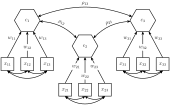
A composite is typically a linear combination of observable random variables.[9] However, also so-called second-order composites as linear combinations of latent variables are conceivable.[8][10]

For a random column vector ${\displaystyle \mathbf {x} }$ of observable variables that is partitioned into sub-vectors ${\displaystyle \mathbf {x} _{i}}$, composites can be defined as weighted linear combinations. So the i-th composite ${\displaystyle c_{i}}$ equals:

${\displaystyle c_{i}=\mathbf {w} _{i}'\mathbf {x} _{i}}$,

where the weights of each composite are appropriately normalized (see Confirmatory composite analysis#Model identification). In the following, it is assumed that the weights are scaled in such a way that each composite has a variance of one, i.e., ${\displaystyle \mathbf {w} _{i}'\mathbf {\Sigma } _{ii}\mathbf {w} _{i}}$. Moreover, without loss of generality, it is assumed that the observable random variables are standardized having a mean of zero and a unit variance. Generally, the variance-covariance matrices ${\displaystyle \mathbf {\Sigma } _{ii}}$ of the sub-vectors are not constrained beyond being positive definite. Similar to the latent variables of a factor model, the composites explain the covariances between the sub-vectors leading to the following inter-block covariance matrix:

${\displaystyle \mathbf {\Sigma } _{ij}=\rho _{ij}\mathbf {\Sigma } _{ii}\mathbf {w} _{i}(\mathbf {\Sigma } _{jj}\mathbf {w} _{j})'}$,

where ${\displaystyle \rho _{ij}}$ is the correlation between the composites ${\displaystyle c_{j}}$ and ${\displaystyle c_{i}}$. The composite model imposes rank one constraints on the inter-block covariance matrices ${\displaystyle \mathbf {\Sigma } _{ij}}$, i.e., ${\displaystyle {\text{rank}}(\mathbf {\Sigma } _{ij})=1}$. Generally, the variance-covariance matrix of ${\displaystyle \mathbf {x} }$ is positive definite iff the correlation matrix of the composites ${\displaystyle \mathbf {R} :=(\rho _{ij})}$ and the variance-covarianc matrices ${\displaystyle \mathbf {\Sigma } _{jj}}$'s are both positive definite.[6]

In addition, the composites can be related via a structural model which constrains the correlation matrix ${\displaystyle \mathbf {R} }$ indirectly via a set of simultaneous equations:[6]

${\displaystyle \mathbf {B} \mathbf {c} _{\text{endogenous}}=\mathbf {C} \mathbf {c} _{\text{exogenous}}+\mathbf {z} }$,

where the vector ${\displaystyle \mathbf {c} }$ is partitioned in an exogenous and an endogenous part, and the matrices ${\displaystyle \mathbf {B} }$ and ${\displaystyle \mathbf {C} }$ contain the so-called path (and feedback) coefficients. Moreover, the vector ${\displaystyle \mathbf {z} }$ contains the structural error terms having a zero mean and being uncorrelated with ${\displaystyle \mathbf {c} _{\text{exogenous}}}$. As the model needs not to be recursive, the matrix ${\displaystyle \mathbf {B} }$ is not necessarily triangular and the elements of ${\displaystyle \mathbf {z} }$ may be correlated.

To ensure identification of the composite model, each composite must be correlated with at least one variable not forming the composite. Additionally to this non-isolation condition, each composite needs to be normalized, e.g., by fixing one weight per composite, the length of each weight vector, or the composite’s variance to a certain value.[1] If the composites are embedded in a structural model, also the structural model needs to be identified.[6] Finally, since the weight signs are still undetermined, it is recommended to select a dominant indicator per block of indicators that dictates the orientation of the composite.[2]

The degrees of freedom of the basic composite model, i.e., with no constraints imposed on the composites' correlation matrix ${\displaystyle \mathbf {R} }$, are calculated as follows:[1]

To estimate a composite model, various methods that create composites can be used[5] such as generalized canonical correlation, principal component analysis, and linear discriminant analysis. Moreover composite-based methods for SEM can be employed to estimate weights and the correlations among the composites such as partial least squares path modeling, and generalized structured component analysis[11].

In CCA, the model fit, i.e., the discrepancy between the estimated model-implied variance-covariance matrix ${\displaystyle {\hat {\mathbf {\Sigma } }}}$ and its sample counterpart ${\displaystyle \mathbf {S} }$, can be assessed in two non-exclusive ways. On the one hand, measures of fit can be employed; on the other hand, a test for overall model fit can be used. While the former relies on heuristic rules, the latter is based on statistical inferences.

Fit measures for composite models comprises statistics such as the standardized root mean square residual (SRMR)[12][3], and the root mean squared error of outer residuals (RMS${\displaystyle _{\theta }}$)[13] In contrast to fit measures for common factor models, fit measures for composite models are relatively unexplored and reliable thresholds still need to be determined. To assess the overall model fit by means of statistical testing, the bootstrap test for overall model fit[14], also known as Bollen-Stine bootstrap test[15], can be used to investigate whether a composite model fits to the data.[3][1]

References

- Schuberth, Florian; Henseler, Jörg; Dijkstra, Theo K. (2018). "Confirmatory Composite Analysis". Frontiers in Psychology. 9: 2541. doi:10.3389/fpsyg.2018.02541. PMC 6300521. PMID 30618962.
- Henseler, Jörg; Hubona, Geoffrey; Ray, Pauline Ash (2016). "Using PLS path modeling in new technology research: updated guidelines". Industrial Management & Data Systems. 116 (1): 2–20. doi:10.1108/IMDS-09-2015-0382.
- Henseler, Jörg; Dijkstra, Theo K.; Sarstedt, Marko; Ringle, Christian M.; Diamantopoulos, Adamantios; Straub, Detmar W.; Ketchen, David J.; Hair, Joseph F.; Hult, G. Tomas M.; Calantone, Roger J. (2014). "Common Beliefs and Reality About PLS". Organizational Research Methods. 17 (2): 182–209. doi:10.1177/1094428114526928.
- Dijkstra, Theo K. (2010). "Latent Variables and Indices: Herman Wold's Basic Design and Partial Least Squares". In Esposito Vinzi, Vincenzo; Chin, Wynne W.; Henseler, Jörg; Wang, Huiwen (eds.). Handbook of Partial Least Squares. Berlin, Heidelberg: Springer Handbooks of Computational Statistics. pp. 23–46. CiteSeerX 10.1.1.579.8461. doi:10.1007/978-3-540-32827-8_2. ISBN 978-3-540-32825-4.
- Dijkstra, Theo K.; Henseler, Jörg (2011). "Linear indices in nonlinear structural equation models: best fitting proper indices and other composites". Quality & Quantity. 45 (6): 1505–1518. doi:10.1007/s11135-010-9359-z.
- Dijkstra, Theo K. (2017). "A Perfect Match Between a Model and a Mode". In Latan, Hengky; Noonan, Richard (eds.). Partial Least Squares Path Modeling: Basic Concepts, Methodological Issues and Applications. Cham: Springer International Publishing. pp. 55–80. doi:10.1007/978-3-319-64069-3_4. ISBN 978-3-319-64068-6.
- Simon, Herbert A. (1969). The sciences of the artificial (3rd ed.). Cambridge, MA: MIT Press.
- Henseler, Jörg (2017). "Bridging Design and Behavioral Research With Variance-Based Structural Equation Modeling" (PDF). Journal of Advertising. 46 (1): 178–192. doi:10.1080/00913367.2017.1281780.
- Bollen, Kenneth A.; Bauldry, Shawn (2011). "Three Cs in measurement models: Causal indicators, composite indicators, and covariates". Psychological Methods. 16 (3): 265–284. doi:10.1037/a0024448. PMC 3889475. PMID 21767021.
- van Riel, Allard C. R.; Henseler, Jörg; Kemény, Ildikó; Sasovova, Zuzana (2017). "Estimating hierarchical constructs using consistent partial least squares: The case of second-order composites of common factors". Industrial Management & Data Systems. 117 (3): 459–477. doi:10.1108/IMDS-07-2016-0286.
- Hwang, Heungsun; Takane, Yoshio (March 2004). "Generalized structured component analysis". Psychometrika. 69 (1): 81–99. doi:10.1007/BF02295841.
- Hu, Li-tze; Bentler, Peter M. (1998). "Fit indices in covariance structure modeling: Sensitivity to underparameterized model misspecification". Psychological Methods. 3 (4): 424–453. doi:10.1037/1082-989X.3.4.424.
- Lohmöller, Jan-Bernd (1989). Latent Variable Path Modeling with Partial Least Squares. Physica-Verlag Heidelberg. ISBN 9783642525148.
- Beran, Rudolf; Srivastava, Muni S. (1985). "Bootstrap Tests and Confidence Regions for Functions of a Covariance Matrix". The Annals of Statistics. 13 (1): 95–115. doi:10.1214/aos/1176346579.
- Bollen, Kenneth A.; Stine, Robert A. (1992). "Bootstrapping Goodness-of-Fit Measures in Structural Equation Models". Sociological Methods & Research. 21 (2): 205–229. doi:10.1177/0049124192021002004.