Bethe–Salpeter equation
The Bethe–Salpeter equation (named after Hans Bethe and Edwin Salpeter)[1] describes the bound states of a two-body (particles) quantum field theoretical system in a relativistically covariant formalism. The equation was actually first published in 1950 at the end of a paper by Yoichiro Nambu, but without derivation.[2]
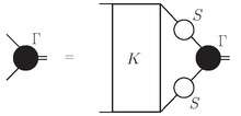
Due to its generality and its application in many branches of theoretical physics, the Bethe–Salpeter equation appears in many different forms. One form, that is quite often used in high energy physics is

where Γ is the Bethe–Salpeter amplitude, K the interaction and S the propagators of the two participating particles.
In quantum theory, bound states are objects that live for an infinite time (otherwise they are called resonances), thus the constituents interact infinitely many times. By summing up, infinitely many times, all possible interactions that can occur between the two constituents, the Bethe–Salpeter equation is a tool to calculate properties of bound states. Its solution, the Bethe–Salpeter amplitude, is a description of the bound state under consideration.
As it can be derived via identifying bound-states with poles in the S-matrix, it can be connected to the quantum theoretical description of scattering processes and Green's functions.
The Bethe–Salpeter equation is a general quantum field theoretical tool, thus applications for it can be found in any quantum field theory. Some examples are positronium (bound state of an electron–positron pair), excitons (bound state of an electron–hole pair[3]), and mesons (as quark-antiquark bound-state).[4]
Even for simple systems such as the positronium, the equation cannot be solved exactly, although in principle it can be formulated exactly. A classification of the states can be achieved without the need for an exact solution. If one of the particles is significantly more massive than the other, the problem is considerably simplified as one solves the Dirac equation for the lighter particle under the external potential of the heavier particle.
Derivation
The starting point for the derivation of the Bethe–Salpeter equation is the two-particle (or four point) Dyson equation

in momentum space, where "G" is the two-particle Green function , "S" are the free propagators and "K" is an interaction kernel, which contains all possible interaction between the two particles. The crucial step is now, to assume that bound states appear as poles in the Green function. One assumes, that two particles come together and form a bound state with mass "M", this bound state propagates freely, and then the bound state splits in its two constituents again. Therefore, one introduces the Bethe–Salpeter wave function , which is a transition amplitude of two constituents into a bound state , and then makes an ansatz for the Green function in the vicinity of the pole as


where P is the total momentum of the system. One sees, that if for this momentum the equation holds, what is exactly the Einstein energy-momentum relation (with the Four-momentum and ) the four-point Green function contains a pole. If one plugs that ansatz into the Dyson equation above, and sets the total momentum "P" such that the energy-momentum relation holds, on both sides of the term a pole appears.


Comparing the residues yields

This is already the Bethe–Salpeter equation, written in terms of the Bethe–Salpeter wave functions. To obtain the above form one introduces the Bethe–Salpeter amplitudes "Γ"

and gets finally

which is written down above, with the explicit momentum dependence.
Rainbow-ladder approximation
In principle the interaction kernel K contains all possible two-particle-irreducible interactions that can occur between the two constituents. Thus, in practical calculations one has to model it and only choose a subset of the interactions. As in quantum field theories, interaction is described via the exchange of particles (e.g. photons in quantum electrodynamics, or gluons in quantum chromodynamics), the most simple interaction is the exchange of only one of these force-particles.
As the Bethe–Salpeter equation sums up the interaction infinitely many times, the resulting Feynman graph has the form of a ladder (or rainbow).
While in quantum electrodynamics the ladder approximation caused problems with crossing symmetry and gauge invariance and thus crossed ladder terms had to be included, in quantum chromodynamics this approximation is used phenomenologically quite a lot to calculate hadron masses,[4] since it respects Chiral symmetry breaking and therefore is an important part of the generation of these masses.
Normalization
As for any homogeneous equation, the solution of the Bethe–Salpeter equation is determined only up to a numerical factor. This factor has to be specified by a certain normalization condition. For the Bethe–Salpeter amplitudes this is usually done by demanding probability conservation (similar to the normalization of the quantum mechanical Wave function), which corresponds to the equation [5]

Normalizations to the charge and energy-momentum tensor of the bound state lead to the same equation. In ladder approximation the Interaction kernel does not depend on the total momentum of the Bethe–Salpeter amplitude, thus, for this case, the second term of the normalization condition vanishes.
See also
- ABINIT – plane wave
- Araki–Sucher correction
- Breit equation
- Lippmann–Schwinger equation
- Schwinger–Dyson equation
- Two-body Dirac equations
- YAMBO code – plane wave
References
- H. Bethe, E. Salpeter (1951). "A Relativistic Equation for Bound-State Problems". Physical Review. 84 (6): 1232. Bibcode:1951PhRv...84.1232S. doi:10.1103/PhysRev.84.1232.
- Y. Nambu (1950). "Force Potentials in Quantum Field Theory". Progress of Theoretical Physics. 5 (4): 614. doi:10.1143/PTP.5.614.
- M. S. Dresselhaus; et al. (2007). "Exciton Photophysics of Carbon Nanotubes". Annual Review of Physical Chemistry. 58: 719. Bibcode:2007ARPC...58..719D. doi:10.1146/annurev.physchem.58.032806.104628.
- P. Maris and P. Tandy (2006). "QCD modeling of hadron physics". Nuclear Physics B. 161: 136. arXiv:nucl-th/0511017. Bibcode:2006NuPhS.161..136M. doi:10.1016/j.nuclphysbps.2006.08.012.
- N. Nakanishi (1969). "A general survey of the theory of the Bethe–Salpeter equation". Progress of Theoretical Physics Supplement. 43: 1–81. Bibcode:1969PThPS..43....1N. doi:10.1143/PTPS.43.1.
Bibliography
Many modern quantum field theory textbooks and a few articles provide pedagogical accounts for the Bethe–Salpeter equation's context and uses. See:
- W. Greiner, J. Reinhardt (2003). Quantum Electrodynamics (3rd ed.). Springer. ISBN 978-3-540-44029-1.
- Z.K. Silagadze (1998). "Wick–Cutkosky model: An introduction". arXiv:hep-ph/9803307.
Still a good introduction is given by the review article of Nakanishi
- N. Nakanishi (1969). "A general survey of the theory of the Bethe–Salpeter equation". Progress of Theoretical Physics Supplement. 43: 1–81. Bibcode:1969PThPS..43....1N. doi:10.1143/PTPS.43.1.
For historical aspects, see
- E.E. Salpeter (2008). "Bethe–Salpeter equation (origins)". Scholarpedia. 3 (11): 7483. arXiv:0811.1050. Bibcode:2008SchpJ...3.7483S. doi:10.4249/scholarpedia.7483.
External links
- BerkeleyGW – plane-wave pseudopotential method
- ExC - plane wave
- Fiesta - Gaussian all-electron method