Basis set (chemistry)
A basis set in theoretical and computational chemistry is a set of functions (called basis functions) that is used to represent the electronic wave function in the Hartree–Fock method or density-functional theory in order to turn the partial differential equations of the model into algebraic equations suitable for efficient implementation on a computer.
The use of basis sets is equivalent to the use of an approximate resolution of the identity. The single-particle states (molecular orbitals) are then expressed as linear combinations of the basis functions.
The basis set can either be composed of atomic orbitals (yielding the linear combination of atomic orbitals approach), which is the usual choice within the quantum chemistry community, or plane waves which are typically used within the solid state community. Several types of atomic orbitals can be used: Gaussian-type orbitals, Slater-type orbitals, or numerical atomic orbitals. Out of the three, Gaussian-type orbitals are by far the most often used, as they allow efficient implementations of Post-Hartree–Fock methods.
Introduction
In modern computational chemistry, quantum chemical calculations are performed using a finite set of basis functions. When the finite basis is expanded towards an (infinite) complete set of functions, calculations using such a basis set are said to approach the complete basis set (CBS) limit. In this article, basis function and atomic orbital are sometimes used interchangeably, although the basis functions are usually not true atomic orbitals, because many basis functions are used to describe polarization effects in molecules.
Within the basis set, the wavefunction is represented as a vector, the components of which correspond to coefficients of the basis functions in the linear expansion. In such a basis, one-electron operators correspond to matrices (a.k.a. rank two tensors), whereas two-electron operators are rank four tensors.
When molecular calculations are performed, it is common to use a basis composed of atomic orbitals, centered at each nucleus within the molecule (linear combination of atomic orbitals ansatz). The physically best motivated basis set are Slater-type orbitals (STOs), which are solutions to the Schrödinger equation of hydrogen-like atoms, and decay exponentially far away from the nucleus. It can be shown that the molecular orbitals of Hartree-Fock and density-functional theory also exhibit exponential decay. Furthermore, S-type STOs also satisfy Kato's cusp condition at the nucleus, meaning that they are able to accurately describe electron density near the nucleus. However, hydrogen-like atoms lack many-electron interactions, thus the orbitals do not accurately describe electron state correlations.
Unfortunately, calculating integrals with STOs is computationally difficult and it was later realized by Frank Boys that STOs could be approximated as linear combinations of Gaussian-type orbitals (GTOs) instead. Because the product of two GTOs can be written as a linear combination of GTOs, integrals with Gaussian basis functions can be written in closed form, which leads to huge computational savings (see John Pople).
Dozens of Gaussian-type orbital basis sets have been published in the literature.[1] Basis sets typically come in hierarchies of increasing size, giving a controlled way to obtain more accurate solutions, however at a higher cost.
The smallest basis sets are called minimal basis sets. A minimal basis set is one in which, on each atom in the molecule, a single basis function is used for each orbital in a Hartree–Fock calculation on the free atom. For atoms such as lithium, basis functions of p type are also added to the basis functions that correspond to the 1s and 2s orbitals of the free atom, because lithium also has a 1s2p bound state. For example, each atom in the second period of the periodic system (Li - Ne) would have a basis set of five functions (two s functions and three p functions).
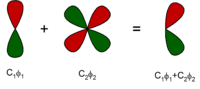
The minimal basis set is close to exact for the gas-phase atom. In the next level, additional functions are added to describe polarization of the electron density of the atom in molecules. These are called polarization functions. For example, while the minimal basis set for hydrogen is one function approximating the 1s atomic orbital, a simple polarized basis set typically has two s- and one p-function (which consists of three basis functions: px, py and pz). This adds flexibility to the basis set, effectively allowing molecular orbitals involving the hydrogen atom to be more asymmetric about the hydrogen nucleus. This is very important for modeling chemical bonding, because the bonds are often polarized. Similarly, d-type functions can be added to a basis set with valence p orbitals, and f-functions to a basis set with d-type orbitals, and so on.
Another common addition to basis sets is the addition of diffuse functions. These are extended Gaussian basis functions with a small exponent, which give flexibility to the "tail" portion of the atomic orbitals, far away from the nucleus. Diffuse basis functions are important for describing anions or dipole moments, but they can also be important for accurate modeling of intra- and intermolecular bonding.
Minimal basis sets
The most common minimal basis set is STO-nG, where n is an integer. This n value represents the number of Gaussian primitive functions comprising a single basis function. In these basis sets, the same number of Gaussian primitives comprise core and valence orbitals. Minimal basis sets typically give rough results that are insufficient for research-quality publication, but are much cheaper than their larger counterparts. Commonly used minimal basis sets of this type are:
- STO-3G
- STO-4G
- STO-6G
- STO-3G* - Polarized version of STO-3G
There are several other minimum basis sets that have been used such as the MidiX basis sets.
Split-valence basis sets
During most molecular bonding, it is the valence electrons which principally take part in the bonding. In recognition of this fact, it is common to represent valence orbitals by more than one basis function (each of which can in turn be composed of a fixed linear combination of primitive Gaussian functions). Basis sets in which there are multiple basis functions corresponding to each valence atomic orbital are called valence double, triple, quadruple-zeta, and so on, basis sets (zeta, ζ, was commonly used to represent the exponent of an STO basis function[3]). Since the different orbitals of the split have different spatial extents, the combination allows the electron density to adjust its spatial extent appropriate to the particular molecular environment. In contrast, minimal basis sets lack the flexibility to adjust to different molecular environments.
Pople basis sets
The notation for the split-valence basis sets arising from the group of John Pople is typically X-YZg.[4] In this case, X represents the number of primitive Gaussians comprising each core atomic orbital basis function. The Y and Z indicate that the valence orbitals are composed of two basis functions each, the first one composed of a linear combination of Y primitive Gaussian functions, the other composed of a linear combination of Z primitive Gaussian functions. In this case, the presence of two numbers after the hyphens implies that this basis set is a split-valence double-zeta basis set. Split-valence triple- and quadruple-zeta basis sets are also used, denoted as X-YZWg, X-YZWVg, etc. Here is a list of commonly used split-valence basis sets of this type:
- 3-21G
- 3-21G* - Polarization functions on heavy atoms
- 3-21G** - Polarization functions on heavy atoms and hydrogen
- 3-21+G - Diffuse functions on heavy atoms
- 3-21++G - Diffuse functions on heavy atoms and hydrogen
- 3-21+G* - Polarization and diffuse functions on heavy atoms
- 3-21+G** - Polarization functions on heavy atoms and hydrogen, as well as diffuse functions on heavy atoms
- 4-21G
- 4-31G
- 6-21G
- 6-31G
- 6-31G*
- 6-31+G*
- 6-31G(3df, 3pd)
- 6-311G
- 6-311G*
- 6-311+G*
The 6-31G* basis set (defined for the atoms H through Zn) is a valence double-zeta polarized basis set that adds to the 6-31G set five d-type Cartesian-Gaussian polarization functions on each of the atoms Li through Ca and ten f-type Cartesian Gaussian polarization functions on each of the atoms Sc through Zn.
Pople basis sets are somewhat outdated, as correlation-consistent or polarization-consistent basis sets typically yield better results with similar resources. Also note that some Pople basis sets have grave deficiencies that may lead to incorrect results.[5]
Correlation-consistent basis sets
Ones of the most widely used basis sets are those developed by Dunning and coworkers,[6] since they are designed for converging Post-Hartree–Fock calculations systematically to the complete basis set limit using empirical extrapolation techniques.
For first- and second-row atoms, the basis sets are cc-pVNZ where N=D,T,Q,5,6,... (D=double, T=triples, etc.). The 'cc-p', stands for 'correlation-consistent polarized' and the 'V' indicates they are valence-only basis sets. They include successively larger shells of polarization (correlating) functions (d, f, g, etc.). More recently these 'correlation-consistent polarized' basis sets have become widely used and are the current state of the art for correlated or post-Hartree–Fock calculations. Examples of these are:
- cc-pVDZ - Double-zeta
- cc-pVTZ - Triple-zeta
- cc-pVQZ - Quadruple-zeta
- cc-pV5Z - Quintuple-zeta, etc.
- aug-cc-pVDZ, etc. - Augmented versions of the preceding basis sets with added diffuse functions.
- cc-pCVDZ - Double-zeta with core correlation
For period-3 atoms (Al-Ar), additional functions have turned out to be necessary; these are the cc-pV(N+d)Z basis sets. Even larger atoms may employ pseudopotential basis sets, cc-pVNZ-PP, or relativistic-contracted Douglas-Kroll basis sets, cc-pVNZ-DK.
While the usual Dunning basis sets are for valence-only calculations, the sets can be augmented with further functions that describe core electron correlation. These core-valence sets (cc-pCVXZ) can be used to approach the exact solution to the all-electron problem, and they are necessary for accurate geometric and nuclear property calculations.
Weighted core-valence sets (cc-pwCVXZ) have also been recently suggested. The weighted sets aim to capture core-valence correlation, while neglecting most of core-core correlation, in order to yield accurate geometries with smaller cost than the cc-pCVXZ sets.
Diffuse functions can also be added for describing anions and long-range interactions such as Van der Waals forces, or to perform electronic excited-state calculations, electric field property calculations. A recipe for constructing additional augmented functions exists; as many as five augmented functions have been used in second hyperpolarizability calculations in the literature. Because of the rigorous construction of these basis sets, extrapolation can be done for almost any energetic property. However, care must be taken when extrapolating energy differences as the individual energy components converge at different rates: the Hartree-Fock energy converges exponentially, whereas the correlation energy converges only polynomially.
| H-He | Li-Ne | Na-Ar | |
|---|---|---|---|
| cc-pVDZ | [2s1p] → 5 func. | [3s2p1d] → 14 func. | [4s3p1d] → 18 func. |
| cc-pVTZ | [3s2p1d] → 14 func. | [4s3p2d1f] → 30 func. | [5s4p2d1f] → 34 func. |
| cc-pVQZ | [4s3p2d1f] → 30 func. | [5s4p3d2f1g] → 55 func. | [6s5p3d2f1g] → 59 func. |
| aug-cc-pVDZ | [3s2p] → 9 func. | [4s3p2d] → 23 func. | [5s4p2d] → 27 func. |
| aug-cc-pVTZ | [4s3p2d] → 23 func. | [5s4p3d2f] → 46 func. | [6s5p3d2f] → 50 func. |
| aug-cc-pVQZ | [5s4p3d2f] → 46 func. | [6s5p4d3f2g] → 80 func. | [7s6p4d3f2g] → 84 func. |
To understand how to get the number of functions take the cc-pVDZ basis set for H: There are two s (L = 0) orbitals and one p (L = 1) orbital that has 3 components along the z-axis (mL = -1,0,1) corresponding to px, py and pz. Thus, five spatial orbitals in total. Note that each orbital can hold two electrons of opposite spin.
For example, Ar [1s, 2s, 2p, 3s, 3p] has 3 s orbitals (L=0) and 2 sets of p orbitals (L=1). Using cc-pVDZ, orbitals are [1s, 2s, 2p, 3s, 3s', 3p, 3p', 3d'] (where ' represents the added in polarisation orbitals), with 4 s orbitals (4 basis functions), 3 sets of p orbitals (3 × 3 = 9 basis functions), and 1 set of d orbitals (5 basis functions). Adding up the basis functions gives a total of 18 functions for Ar with the cc-pVDZ basis-set.
Polarization-consistent basis sets
Density-functional theory has recently become widely used in computational chemistry. However, the correlation-consistent basis sets described above are suboptimal for density-functional theory, because the correlation-consistent sets have been designed for Post-Hartree–Fock, while density-functional theory exhibits much more rapid basis set convergence than wave function methods.
Adopting a similar methodology to the correlation-consistent series, Frank Jensen introduced polarization-consistent (pc-n) basis sets as a way to quickly converge density functional theory calculations to the complete basis set limit.[7] Like the Dunning sets, the pc-n sets can be combined with basis set extrapolation techniques to obtain CBS values.
The pc-n sets can be augmented with diffuse functions to obtain augpc-n sets.
Karlsruhe basis sets
Some of the various valence adaptations of Karlsruhe basis sets are
- def2-SV(P) - Split valence with polarization functions on heavy atoms (not hydrogen)
- def2-SVP - Split valence polarization
- def2-SVPD - Split valence polarization with diffuse functions
- def2-TZVP - Valence triple-zeta polarization
- def2-TZVPD - Valence triple-zeta polarization with diffuse functions
- def2-TZVPP - Valence triple-zeta with two sets of polarization functions
- def2-TZVPPD - Valence triple-zeta with two sets of polarization functions and a set of diffuse functions
- def2-QZVP - Valence quadruple-zeta polarization
- def2-QZVPD - Valence quadruple-zeta polarization with diffuse functions
- def2-QZVPP - Valence quadruple-zeta with two sets of polarization functions
- def2-QZVPPD - Valence quadruple-zeta with two sets of polarization functions and a set of diffuse functions
Completeness-optimized basis sets
Gaussian-type orbital basis sets are typically optimized to reproduce the lowest possible energy for the systems used to train the basis set. However, the convergence of the energy does not imply convergence of other properties, such as nuclear magnetic shieldings, the dipole moment, or the electron momentum density, which probe different aspects of the electronic wave function.
Manninen and Vaara have proposed completeness-optimized basis sets,[8] where the exponents are obtained by maximization of the one-electron completeness profile[9] instead of minimization of the energy. Completeness-optimized basis sets are a way to easily approach the complete basis set limit of any property at any level of theory, and the procedure is simple to automatize.[10]
Completeness-optimized basis sets are tailored to a specific property. This way, the flexibility of the basis set can be focused on the computational demands of the chosen property, typically yielding much faster convergence to the complete basis set limit than is achievable with energy-optimized basis sets.
Plane-wave basis sets
In addition to localized basis sets, plane-wave basis sets can also be used in quantum-chemical simulations. Typically, the choice of the plane wave basis set is based on a cutoff energy. The plane waves in the simulation cell that fit below the energy criterion are then included in the calculation. These basis sets are popular in calculations involving three-dimensional periodic boundary conditions.
The main advantage of a plane-wave basis is that it is guaranteed to converge in a smooth, monotonic manner to the target wavefunction. In contrast, when localized basis sets are used, monotonic convergence to the basis set limit may be difficult due to problems with over-completeness: in a large basis set, functions on different atoms start to look alike, and many eigenvalues of the overlap matrix approach zero.
In addition, certain integrals and operations are much easier to program and carry out with plane-wave basis functions than with their localized counterparts. For example, the kinetic energy operator is diagonal in the reciprocal space. Integrals over real-space operators can be efficiently carried out using fast Fourier transforms. The properties of the Fourier Transform allow a vector representing the gradient of the total energy with respect to the plane-wave coefficients to be calculated with a computational effort that scales as NPW*ln(NPW) where NPW is the number of plane-waves. When this property is combined with separable pseudopotentials of the Kleinman-Bylander type and pre-conditioned conjugate gradient solution techniques, the dynamic simulation of periodic problems containing hundreds of atoms becomes possible.
In practice, plane-wave basis sets are often used in combination with an 'effective core potential' or pseudopotential, so that the plane waves are only used to describe the valence charge density. This is because core electrons tend to be concentrated very close to the atomic nuclei, resulting in large wavefunction and density gradients near the nuclei which are not easily described by a plane-wave basis set unless a very high energy cutoff, and therefore small wavelength, is used. This combined method of a plane-wave basis set with a core pseudopotential is often abbreviated as a PSPW calculation.
Furthermore, as all functions in the basis are mutually orthogonal and are not associated with any particular atom, plane-wave basis sets do not exhibit basis-set superposition error. However, the plane-wave basis set is dependent on the size of the simulation cell, complicating cell size optimization.
Due to the assumption of periodic boundary conditions, plane-wave basis sets are less well suited to gas-phase calculations than localized basis sets. Large regions of vacuum need to be added on all sides of the gas-phase molecule in order to avoid interactions with the molecule and its periodic copies. However, the plane waves use a similar accuracy to describe the vacuum region as the region where the molecule is, meaning that obtaining the truly noninteracting limit may be computationally costly.
Real-space basis sets
Analogous to the plane wave basis sets, where the basis functions are eigenfunctions of the momentum operator, there are basis sets whose functions are eigenfunctions of the position operator, that is, points on a uniform mesh in real space. The actual implementation may use finite differences, finite elements or Lagrange sinc-functions, or wavelets.
Since functions form an orthonormal, analytical, and complete basis set. The convergence to the complete basis set limit is systematic and relatively simple. Similarly to plane wave basis sets, the accuracy of sinc basis sets is controlled by an energy cutoff criterion.
In the case of wavelets and finite elements, it is possible to make the mesh adaptive, so that more points are used close to the nuclei. Wavelets rely on the use of localized functions that allow for the development of linear-scaling methods.
Even-tempered basis sets
In 1974 Bardo and Ruedenberg [11] proposed a simple scheme to generate the exponents of a basis set that spans the Hilbert space evenly [12] by following a geometric progression of the form:

for each angular momentum , where is the number of primitives functions. Here, only the two parameters and must be optimized, significantly reducing the dimension of the search space or even avoiding the exponent optimization problem. In order to properly describe electronic delocalized states, a previously optimized standard basis set can be complemented with additional delocalized Gaussian functions with small exponent values, generated by the even-tempered scheme.[12] This approach has also been employed to generate basis sets for other types of quantum particles rather than electrons, like quantum nuclei,[13] negative muons[14] or positrons.[15]


See also
- Basis set superposition error
- Angular momentum
- Atomic orbitals
- Molecular orbitals
- List of quantum chemistry and solid state physics software
References
- Jensen, Frank (2013). "Atomic orbital basis sets". WIREs Comput. Mol. Sci. 3 (3): 273–295. doi:10.1002/wcms.1123.
- Errol G. Lewars (2003-01-01). Computational Chemistry: Introduction to the Theory and Applications of Molecular and Quantum Mechanics (1st ed.). Springer. ISBN 978-1402072857.
- Davidson, Ernest; Feller, David (1986). "Basis set selection for molecular calculations". Chem. Rev. 86 (4): 681–696. doi:10.1021/cr00074a002.
- Ditchfield, R; Hehre, W.J; Pople, J. A. (1971). "Self-Consistent Molecular-Orbital Methods. IX. An Extended Gaussian-Type Basis for Molecular-Orbital Studies of Organic Molecules". J. Chem. Phys. 54 (2): 724–728. Bibcode:1971JChPh..54..724D. doi:10.1063/1.1674902.
- Moran, Damian; Simmonett, Andrew C.; Leach, Franklin E. III; Allen, Wesley D.; Schleyer, Paul v. R.; Schaefer, Henry F. (2006). "Popular theoretical methods predict benzene and arenes to be nonplanar". J. Am. Chem. Soc. 128 (29): 9342–9343. doi:10.1021/ja0630285. PMID 16848464.
- Dunning, Thomas H. (1989). "Gaussian basis sets for use in correlated molecular calculations. I. The atoms boron through neon and hydrogen". J. Chem. Phys. 90 (2): 1007–1023. Bibcode:1989JChPh..90.1007D. doi:10.1063/1.456153.
- Jensen, Frank (2001). "Polarization consistent basis sets: Principles". J. Chem. Phys. 115 (20): 9113–9125. Bibcode:2001JChPh.115.9113J. doi:10.1063/1.1413524.
- Manninen, Pekka; Vaara, Juha (2006). "Systematic Gaussian basis-set limit using completeness-optimized primitive sets. A case for magnetic properties". J. Comput. Chem. 27 (4): 434–445. doi:10.1002/jcc.20358. PMID 16419020.
- Chong, Delano P. (1995). "Completeness profiles of one-electron basis sets". Can. J. Chem. 73 (1): 79–83. doi:10.1139/v95-011.
- Lehtola, Susi (2015). "Automatic algorithms for completeness-optimization of Gaussian basis sets". J. Comput. Chem. 36 (5): 335–347. doi:10.1002/jcc.23802. PMID 25487276.
- Bardo, Richard D.; Ruedenberg, Klaus (February 1974). "Even‐tempered atomic orbitals. VI. Optimal orbital exponents and optimal contractions of Gaussian primitives for hydrogen, carbon, and oxygen in molecules". The Journal of Chemical Physics. 60 (3): 918–931. doi:10.1063/1.1681168. ISSN 0021-9606.
- Cherkes, Ira; Klaiman, Shachar; Moiseyev, Nimrod (2009-11-05). "Spanning the Hilbert space with an even tempered Gaussian basis set". International Journal of Quantum Chemistry. 109 (13): 2996–3002. doi:10.1002/qua.22090.
- Nakai, Hiromi (2002). "Simultaneous determination of nuclear and electronic wave functions without Born-Oppenheimer approximation: Ab initio NO+MO/HF theory". International Journal of Quantum Chemistry. 86 (6): 511–517. doi:10.1002/qua.1106. ISSN 0020-7608.
- Moncada, Félix; Cruz, Daniel; Reyes, Andrés (June 2012). "Muonic alchemy: Transmuting elements with the inclusion of negative muons". Chemical Physics Letters. 539–540: 209–213. Bibcode:2012CPL...539..209M. doi:10.1016/j.cplett.2012.04.062.
- Reyes, Andrés; Moncada, Félix; Charry, Jorge (2019-01-15). "The any particle molecular orbital approach: A short review of the theory and applications". International Journal of Quantum Chemistry. 119 (2): e25705. doi:10.1002/qua.25705. ISSN 0020-7608.
All the many basis sets discussed here along with others are discussed in the references below which themselves give references to the original journal articles:
- Levine, Ira N. (1991). Quantum Chemistry. Englewood Cliffs, New jersey: Prentice Hall. pp. 461–466. ISBN 978-0-205-12770-2.
- Cramer, Christopher J. (2002). Essentials of Computational Chemistry. Chichester: John Wiley & Sons, Ltd. pp. 154–168. ISBN 978-0-471-48552-0.
- Jensen, Frank (1999). Introduction to Computational Chemistry. John Wiley and Sons. pp. 150–176. ISBN 978-0471980858.
- Leach, Andrew R. (1996). Molecular Modelling: Principles and Applications. Singapore: Longman. pp. 68–77. ISBN 978-0-582-23933-3.
- Hehre, Warren J.. (2003). A Guide to Molecular Mechanics and Quantum Chemical Calculations. Irvine, California: Wavefunction, Inc. pp. 40–47. ISBN 978-1-890661-18-2.
- https://web.archive.org/web/20070830043639/http://www.chem.swin.edu.au/modules/mod8/basis1.html
- Moran, Damian; Simmonett, Andrew C.; Leach, Franklin E.; Allen, Wesley D.; Schleyer, Paul v. R.; Schaefer, Henry F. (2006). "Popular Theoretical Methods Predict Benzene and Arenes To Be Nonplanar". Journal of the American Chemical Society. 128 (29): 9342–3. doi:10.1021/ja0630285. PMID 16848464.
- Choi, Sunghwan; Kwangwoo, Hong; Jaewook, Kim; Woo Youn, Kim (2015). "Accuracy of Lagrange-sinc functions as a basis set for electronic structure calculations of atoms and molecules". The Journal of Chemical Physics. 142 (9): 094116. Bibcode:2015JChPh.142i4116C. doi:10.1063/1.4913569. PMID 25747070.
External links
- EMSL Basis Set Exchange
- TURBOMOLE basis set library
- CRYSTAL - Basis Sets Library
- Dyall Basis Sets Library
- Peterson Group Correlation Consistent Basis Sets
- Sapporo Segmented Gaussian Basis Sets Library
- Stuttgart/Cologne energy-consistent (ab initio) pseudopotentials Library
- ChemViz - Basis Sets Lab Activity