Amortized analysis

Amortized analysis of the push operation for a dynamic array

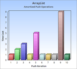
Consider a dynamic array that grows in size as more elements are added to it, such as ArrayList in Java or std::vector in C++. If we started out with a dynamic array of size 4, we could push 4 elements onto it, and each operation would take constant time. Yet pushing a fifth element onto that array would take longer as the array would have to create a new array of double the current size (8), copy the old elements onto the new array, and then add the new element. The next three push operations would similarly take constant time, and then the subsequent addition would require another slow doubling of the array size.

In general if we consider an arbitrary number of pushes n + 1 to an array of size n, we notice that push operations take constant time except for the last one which takes ${\displaystyle \Theta (n)}$ time to perform the size doubling operation. Since there were n + 1 operations total we can take the average of this and find that pushing elements onto the dynamic array takes: ${\displaystyle {\tfrac {n\Theta (1)+\Theta (n)}{n+1}}=\Theta (1)}$, constant time.[4]

Shown is a Ruby implementation of a Queue, a FIFO data structure:

class Queue
  def initialize
    @input = []
    @output = []
  end

  def enqueue(element)
    @input << element
  end

  def dequeue
    if @output.empty?
      while @input.any?
        @output << @input.pop
      end
    end

    @output.pop
  end
end

The enqueue operation just pushes an element onto the input array; this operation does not depend on the lengths of either input or output and therefore runs in constant time.

However the dequeue operation is more complicated. If the output array already has some elements in it, then dequeue runs in constant time; otherwise, dequeue takes ${\displaystyle O(n)}$ time to add all the elements onto the output array from the input array, where n is the current length of the input array. After copying n elements from input, we can perform n dequeue operations, each taking constant time, before the output array is empty again. Thus, we can perform a sequence of n dequeue operations in only ${\displaystyle O(n)}$ time, which implies that the amortized time of each dequeue operation is ${\displaystyle O(1)}$.[5]

Alternatively, we can charge the cost of copying any item from the input array to the output array to the earlier enqueue operation for that item. This charging scheme doubles the amortized time for enqueue but reduces the amortized time for dequeue to ${\displaystyle O(1)}$.

References

- Allan Borodin and Ran El-Yaniv (1998). Online Computation and Competitive Analysis. Cambridge University Press. pp. 20, 141.
- "Lecture 7: Amortized Analysis" (PDF). Carnegie Mellon University. Retrieved 14 March 2015.
- Rebecca Fiebrink (2007), Amortized Analysis Explained (PDF), archived from the original (PDF) on 20 October 2013, retrieved 3 May 2011
- Tarjan, Robert Endre (April 1985). "Amortized Computational Complexity" (PDF). SIAM Journal on Algebraic and Discrete Methods. 6 (2): 306–318. doi:10.1137/0606031.
- Kozen, Dexter (Spring 2011). "CS 3110 Lecture 20: Amortized Analysis". Cornell University. Retrieved 14 March 2015.
- Grossman, Dan. "CSE332: Data Abstractions" (PDF). cs.washington.edu. Retrieved 14 March 2015.