Thomas–Fermi screening

Thomas–Fermi screening is a theoretical approach to calculating the effects of electric field screening by electrons in a solid.^[1] It is a special case of the more general Lindhard theory; in particular, Thomas–Fermi screening is the limit of the Lindhard formula when the wavevector (the reciprocal of the length-scale of interest) is much smaller than the fermi wavevector, i.e. the long-distance limit.^[1] It is named after Llewellyn Thomas and Enrico Fermi.

The Thomas-Fermi wavevector (in Gaussian-cgs units) is^[1]

k_{0}^{2}=4\pi e^{2}{\frac {\partial n}{\partial \mu }}

,

where μ is the chemical potential (fermi level), n is the electron concentration and e is the elementary charge.

Under many circumstances, including semiconductors that are not too heavily doped, n∝e^μ/k_BT, where k_B is Boltzmann constant and T is temperature. In this case,

k_{0}^{2}=4\pi e^{2}n/(k_{\rm {B}}T)

,

i.e. 1/k₀ is given by the familiar formula for Debye length. In the opposite extreme, in the low-temperature limit T=0, electrons behave as quantum particles (Fermions). Such an approximation is valid for metals at room temperature, and the Thomas-Fermi screening wavevector k_TF given in atomic units is

k_{\rm {TF}}^{2}=4\left({\frac {3n}{\pi }}\right)^{1/3}

.

If we restore the electron mass $m_{e}$ and the Planck constant $\hbar$ , the screening wavevector in Gaussian units is $k_{0}^{2}=k_{\rm {TF}}^{2}(m_{e}/\hbar ^{2})$ .

For more details and discussion, including the one-dimensional and two-dimensional cases, see the article: Lindhard theory.

Derivation

Relation between electron density and internal chemical potential

The internal chemical potential (closely related to Fermi level, see below) of a system of electrons describes how much energy is required to put an extra electron into the system, neglecting electrical potential energy. As the number of electrons in the system increases (with fixed temperature and volume), the internal chemical potential increases. This consequence is largely because electrons satisfy the Pauli exclusion principle, only one electron may occupy an energy level and lower-energy electron states are already full, so the new electrons must occupy higher and higher energy states.

The relationship is described by the electron number density $n(\mu )$ , is a function of μ, the internal chemical potential. The exact functional form depends on the system. For example, for a three-dimensional Fermi gas, a noninteracting electron gas, at absolute zero temperature, the relation is $n(\mu )\propto \mu ^{{3/2}}$ .

Proof: Including spin degeneracy,

n=2{\frac {1}{(2\pi )^{3}}}{\frac {4}{3}}\pi k_{\rm {F}}^{3}\quad ,\quad \mu ={\frac {\hbar ^{2}k_{\rm {F}}^{2}}{2m}}.

(in this context—i.e., absolute zero—the internal chemical potential is more commonly called the Fermi energy).

As another example, for an n-type semiconductor at low to moderate electron concentration, $n(\mu )\propto e^{\mu /k_{\rm {B}}T}$ .

Local approximation

The main assumption in the Thomas–Fermi model is that there is an internal chemical potential at each point r that depends only on the electron concentration at the same point r. This behaviour cannot be exactly true because of the Heisenberg uncertainty principle. No electron can exist at a single point; each is spread out into a wavepacket of size ≈ 1 / k_F, where k_F is the Fermi wavenumber, i.e. a typical wavenumber for the states at the Fermi surface. Therefore it cannot be possible to define a chemical potential at a single point, independent of the electron density at nearby points.

Nevertheless, the Thomas-Fermi model is likely to be a reasonably accurate approximation as long as the potential does not vary much over lengths comparable or smaller than 1 / k_F. This length usually corresponds to a few atoms in metals.

Electrons in equilibrium, nonlinear equation

Finally, the Thomas-Fermi model assumes that the electrons are in equilibrium, meaning that the total chemical potential is the same at all points. (In electrochemistry terminology, "the electrochemical potential of electrons is the same at all points". In semiconductor physics terminology, "the Fermi level is flat".) This balance requires that the variations in internal chemical potential are matched by equal and opposite variations in the electric potential energy. This gives rise to the "basic equation of nonlinear Thomas-Fermi theory":^[1]

\rho ^{{{\text{induced}}}}({\mathbf {r}})=-e[n(\mu _{0}+e\phi ({\mathbf {r}}))-n(\mu _{0})]

where n(μ) is the function discussed above (electron density as a function of internal chemical potential), e is the elementary charge, r is the position, and $\rho ^{{{\text{induced}}}}({\mathbf {r}})$ is the induced charge at r. The electric potential $\phi$ is defined in such a way that $\phi ({\mathbf {r}})=0$ at the points where the material is charge-neutral (the number of electrons is exactly equal to the number of ions), and similarly μ₀ is defined as the internal chemical potential at the points where the material is charge-neutral.

Linearization, dielectric function

If the chemical potential does not vary too much, the above equation can be linearized:

\rho ^{{{\text{induced}}}}({\mathbf {r}})\approx -e^{2}{\frac {\partial n}{\partial \mu }}\phi ({\mathbf {r}})

where $\partial n/\partial \mu$ is evaluated at μ₀ and treated as a constant.

This relation can be converted into a wavevector-dependent dielectric function:^[1]

\epsilon ({\mathbf {q}})=1+{\frac {k_{0}^{2}}{q^{2}}}

(cgs-Gaussian)

where

k_{0}={\sqrt {4\pi e^{2}{\frac {\partial n}{\partial \mu }}}}

At long distances (q→0), the dielectric constant approaches infinity, reflecting the fact that charges get closer and closer to perfectly screened as you observe them from further away.

Example: A point charge

If a point charge Q is placed at r=0 in a solid, what field will it produce, taking electron screening into account?

One seeks a self-consistent solution to two equations:

The Thomas–Fermi screening formula gives the charge density at each point r as a function of the potential $\phi(\mathbf{r})$ at that point.
The Poisson equation (derived from Gauss's law) relates the second derivative of the potential to the charge density.

For the nonlinear Thomas-Fermi formula, solving these simultaneously can be difficult, and usually there is no analytical solution. However, the linearized formula has a simple solution:

\phi ({\mathbf {r}})={\frac {Q}{r}}e^{{-k_{0}r}}

(cgs-Gaussian)

With k₀=0 (no screening), this becomes the familiar Coulomb's law.

Note that there may be dielectric permittivity in addition to the screening discussed here; for example due to the polarization of immobile core electrons. In that case, replace Q by Q/ε, where ε is the relative permittivity due to these other contributions.

Fermi gas at arbitrary temperature

Effective temperature for Thomas-Fermi screening. The approximate form is explained in the article, and uses the power p=1.8.

For a three-dimensional Fermi gas (noninteracting electron gas), the screening wavevector $k_{0}$ can be expressed as a function of both temperature and Fermi energy $E_{\rm {F}}$ . The first step is calculating the internal chemical potential $\mu$ , which involves the inverse of a Fermi-Dirac integral,

{\frac {\mu }{k_{\rm {B}}T}}=F_{1/2}^{-1}\left[{2 \over {3\Gamma (3/2)}}\left({E_{\rm {F}} \over T}\right)^{3/2}\right]

.

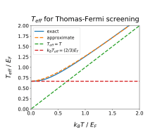
We can express $k_{0}$ in terms of an effective temperature $T_{\rm {eff}}$ : $k_{0}^{2}=4\pi e^{2}n/k_{\rm {B}}T_{\rm {eff}}$ , or $k_{\rm {B}}T_{\rm {eff}}=n\partial \mu /\partial n$ . The general result for $T_{\rm {eff}}$ is

${T_{\rm {eff}} \over T}={4 \over 3\Gamma (1/2)}{(E_{F}/k_{\rm {B}}T)^{3/2} \over F_{-1/2}(\mu /k_{\rm {B}}T)}$ .

In the classical limit $k_{\rm {B}}T\gg E_{\rm {F}}$ , we find $T_{\rm {eff}}=T$ , while in the degenerate limit $k_{\rm {B}}T\ll E_{\rm {F}}$ we find

k_{\rm {B}}T_{\rm {eff}}=(2/3)E_{\rm {F}}

.

A simple approximate form that recovers both limits correctly is

k_{\rm {B}}T_{\rm {eff}}=\left[(k_{\rm {B}}T)^{p}+(2E_{\rm {F}}/3)^{p}\right]^{1/p}

,

for any power $p$ . A value that gives decent agreement with the exact result for all $k_{\rm {B}}T/E_{\rm {F}}$ is $p=1.8$ , which has a maximum relative error of < 2.3%.

References

1 2 3 4 5 N. W. Ashcroft and N. D. Mermin, Solid State Physics (Thomson Learning, Toronto, 1976)

This article is issued from Wikipedia. The text is licensed under Creative Commons - Attribution - Sharealike. Additional terms may apply for the media files.

[Ashcroft-1] 1 2 3 4 5 N. W. Ashcroft and N. D. Mermin, Solid State Physics (Thomson Learning, Toronto, 1976)