Synchronous frame

A reference frame in which the time coordinate defines proper time for all co-moving observers is called "synchronous". It is built by choosing some time-like hypersurface as an origin, such that has in every point a normal along the time line (lies inside the light cone with an apex in that point); all interval elements on this hypersurface are space-like. A family of geodesics normal to this hypersurface are drawn and defined as the time coordinates with a beginning at the hypersurface.

Such a construct, and hence, choice of synchronous frame, is always possible though it is not unique. It allows any transformation of space coordinates that does not depend on time and, additionally, a transformation brought about by the arbitrary choice of hypersurface used for this geometric construct.

Synchronization over a curved space

Synchronization of clocks located at different space points means that events happening at different places can be measured as simultaneous if those clocks show the same times. In the special relativity theory, the space distance element dl is defined as the intervals between two very close events that occur at the same moment of time. In the general relativity theory this cannot be done, that is, one cannot define dl by just substituting dx⁰ = 0 in the metric. The reason for this is the different dependence between proper time and time coordinate x⁰ in different points of space.

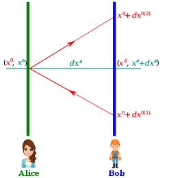
Figure 1. Synchronization of clocks in curved space through light signals.

To find dl in this case, one can first synchronize time over the whole space in the following way (Fig. 1): Bob sends a light signal from some space point B with coordinates x^α + dx^α to Alice who is at a very close point A with coordinates x^α and then Alice immediately reflects the signal back to Bob. The time necessary for this operation (measured by Bob), multiplied by c is, obviously, the doubled distance between Alice and Bob.

The squared interval, with separated space and time coordinates, is:

$ds^{2}=g_{\alpha \beta }\,dx^{\alpha }\,dx^{\beta }+2g_{0\alpha }\,dx^{0}\,dx^{\alpha }+g_{00}\left(dx^{0}\right)^{2},$

(eq. 1)

where a repeated Greek index within a term means summation by values 1, 2, 3. The interval between the events of signal arrival in point A and its immediate reflection back is zero (two events in the same time at the same point). Equation ds² = 0 solved for dx⁰ gives two roots:

dx^{0(1)}={\frac {1}{g_{00}}}\left(-g_{0\alpha }\,dx^{\alpha }-{\sqrt {\left(g_{0\alpha }g_{0\beta }-g_{\alpha \beta }g_{00}\right)\,dx^{\alpha }\,dx^{\beta }}}\right),

$dx^{0(2)}={\frac {1}{g_{00}}}\left(-g_{0\alpha }\,dx^{\alpha }+{\sqrt {\left(g_{0\alpha }g_{0\beta }-g_{\alpha \beta }g_{00}\right)\,dx^{\alpha }\,dx^{\beta }}}\right),$

(eq. 2)

which correspond to the propagation of the signal in both directions between Alice and Bob. If x⁰ is the moment of arrival/reflection of the signal to/from Alice, the moments of signal departure from Bob and its arrival back to Bob correspond, respectively, to x⁰ + dx^{0 (1)} and x⁰ + dx^{0 (2)}. The thick lines on Fig. 1 are the world lines of Alice and Bob with coordinates x^α and x^α + dx^α, respectively, while the red lines are the world lines of the signals. Fig. 1 supposes that dx^{0 (2)} is positive and dx^{0 (1)} is negative, which, however, is not necessarily the case: dx^{0 (1)} and dx^{0 (2)} may have the same sign. The fact that in the latter case the value x⁰ (Alice) in the moment of signal arrival at Alice's position may be less than the value x⁰ (Bob) in the moment of signal departure from Bob does not contain a contradiction because clocks in different points of space are not supposed to be synchronized. It is clear that the full "time" interval between departure and arrival of the signal in Bob's place is

dx^{0(2)}-dx^{0(1)}={\frac {2}{g_{00}}}{\sqrt {\left(g_{0\alpha }g_{0\beta }-g_{\alpha \beta }g_{00}\right)\,dx^{\alpha }\,dx^{\beta }}}.

The respective proper time interval is obtained from the above relationship by multiplication by ${\sqrt {g_{00}}}/c$ , and the distance dl between the two points – by additional multiplication by c/2. As a result:

$dl^{2}=\left(-g_{\alpha \beta }+{\frac {g_{0\alpha }g_{0\beta }}{g_{00}}}\right)\,dx^{\alpha }\,dx^{\beta }.$

(eq. 3)

This is the required relationship that defines distance through the space coordinate elements.

It is obvious that such synchronization should be done by exchange of light signals between points. Consider again propagation of signals between infinitesimally close points A and B in Fig. 1. The clock reading in B which is simultaneous with the moment x⁰ in A lies in the middle between the moments of sending and receiving the signal in B; this is the moment

x^{0}+\Delta x^{0}=x^{0}+{\tfrac {1}{2}}\left(dx^{0(2)}+dx^{0(1)}\right).

Substitute here eq. 2 to find the difference in "time" x⁰ between two simultaneous events occurring in infinitesimally close points as

$\Delta x^{0}=-{\frac {g_{0\alpha }\,dx^{\alpha }}{g_{00}}}\equiv g_{\alpha }\,dx^{\alpha }.$

(eq. 4)

This relationship allows clock synchronization in any infinitesimally small space volume. By continuing such synchronization further from point A, one can synchronize clocks, that is, determine simultaneity of events along any open line. The synchronization condition can be written in another form by multiplying eq. 4 by g₀₀ and bringing terms to the left hand side

$\Delta x_{0}=g_{0i}dx^{i}=0$

(eq. 5)

or, the "covariant differential" dx₀ between two infinitesimally close points should be zero.

However, it is impossible, in general, to synchronize clocks along a closed contour: starting out along the contour and returning to the starting point one would obtain a Δx⁰ value different from zero. Thus, unambiguous synchronization of clocks over the whole space is impossible. An exception are reference frames in which all components g_0α are zeros.

Note the inability to synchronize all clocks is a property of the reference frame and not of the spacetime itself. It is always possible in infinitely many ways in any gravitational field to choose the reference frame so that the three g_0α become zeros and thus enable a complete synchronization of clocks. To this class are assigned cases where g_0α can be made zeros by a simple change in the time coordinate which does not involve a choice of a system of objects that define the space coordinates.

In the special relativity theory, too, proper time elapses differently for clocks moving relatively to each other. In general relativity, proper time is different even in the same reference frame at different points of space. This means that the interval of proper time between two events occurring at some space point and the time interval between the events simultaneous with those at another space point are, in general, different from one another.

Space metric tensor

Rewrite eq. 3 in the form

$dl^{2}=\gamma _{\alpha \beta }\,dx^{\alpha }\,dx^{\beta },$

(eq. 6)

where

$\gamma _{\alpha \beta }=-g_{\alpha \beta }+{\frac {g_{0\alpha }g_{0\beta }}{g_{00}}}$

(eq. 7)

is the three-dimensional metric tensor that determines the metric, that is, the geometrical properties of space. Equations eq. 7 give the relationships between the metric of the three-dimensional space and the metric of the four-dimensional spacetime.

In general, however, the metric g_ik depends on x⁰ so that the space metric eq. 7 changes with time. Therefore, it doesn't make sense to integrate dl: this integral depends on the choice of world line between the two points on which it is taken. It follows that in general relativity the distance between two bodies cannot be determined in general; this distance is determined only for infinitesimally close points. Distance can be determined also for finite space regions only in such reference frames in which g_ik does not depend on time and therefore the integral ∫dl along the space curve acquires some definite sense.

The tensor –γ_αβ is inverse to the contravariant 3-dimensional tensor g^αβ. Indeed, writing equation g^ikg_kl = $\scriptstyle {\delta _{l}^{i}}$ in components, one has:

g^{\alpha \beta }g_{\beta \gamma }+g^{\alpha 0}g_{0\gamma }=\delta _{\gamma }^{\alpha },

$g^{\alpha \beta }g_{\beta 0}+g^{\alpha 0}g_{00}=0,$

(eqs. 8)

g^{0\beta }g_{\beta 0}+g^{00}g_{00}=1.

Determine g^α0 from the second equation and substitute in the first to obtain

$-g^{\alpha \beta }\gamma _{\beta \gamma }=\delta _{\gamma }^{\alpha },$

(eq. 9)

which was to be demonstrated. This result can be presented otherwise by saying that g^αβ are components of a contravariant 3-dimensional tensor corresponding to metric eq. 7:

$\gamma ^{\alpha \beta }=-g^{\alpha \beta }.$

(eq. 10)

The determinants g and γ composed of elements g_ik and γ_αβ, respectively, are related to each other by the simple relationship:

$-g=g_{00}\gamma .$

(eq. 11)

In many applications, it is convenient to define a 3-dimensional vector g with covariant components

$g_{\alpha }=-{\frac {g_{0\alpha }}{g_{00}}}.$

(eq. 12)

Considering g as a vector in space with metric eq. 7, its contravariant components can be written as g^α = γ^αβg_β. Using eq. 11 and the second of eqs. 8, it is easy to see that

$g^{\alpha }=\gamma ^{\alpha \beta }g_{\beta }=-g^{0\alpha }.$

(eq. 13)

From the third of eqs. 8, it follows

$g^{00}={\frac {1}{g_{00}}}-g_{\alpha }g^{\alpha }.$

(eq. 14)

Synchronous coordinates

As concluded from eq. 5, the condition that allows clock synchronization in different space points is that metric tensor components g_0α are zeros. If, in addition, g₀₀ = 1, then the time coordinate x⁰ = t is the proper time in each space point (with c = 1). A reference frame that satisfies the conditions

$g_{00}=1,\quad g_{0\alpha }=0,$

(eq. 15)

is called synchronous frame. The interval element in this system is given by the expression

$ds^{2}=dt^{2}-g_{\alpha \beta }\,dx^{\alpha }\,dx^{\beta },$

(eq. 16)

with the spatial metric tensor components identical (with opposite sign) to the components g_αβ:

$\gamma _{\alpha \beta }=-g_{\alpha \beta }.$

(eq. 17)

Figure 2. A synchronous reference frame built with the choice of the timelike hypersurface t = const (teal color). Only one spatial coordinate x¹ = x is shown. The four observers have the same proper times x⁰ = t which are normal to the hypersurface in their locally flat spacetimes (shown by the light cones). The unit vector n⁰ = u⁰ = 1 is shown in yellow. There are no spatial components (u^α = 0) so the common proper time is a geodesic line with a beginning at the hypersurface and a positive direction (red arrows).

In synchronous frame time, time lines are normal to the hypersurfaces t = const. Indeed, the unit four-vector normal to such a hypersurface n_i = ∂t/∂xⁱ has covariant components n_α = 0, n₀ = 1. The respective contravariant components with the conditions eq. 15 are again n^α = 0, n⁰ = 1.

The components of the unit normal coincide with those of the four-vector uⁱ = dxⁱ/ds which is tangent to the world line x¹, x², x³ = const. The uⁱ with components u^α = 0, u⁰ = 1 automatically satisfies the geodesic equations:

{\frac {du^{i}}{ds}}+\Gamma _{kl}^{i}u^{k}u^{l}=\Gamma _{00}^{i}=0,

since, from the conditions eq. 15, the Christoffel symbols $\Gamma _{00}^{\alpha }$ and $\Gamma _{00}^{0}$ vanish identically. Therefore, in the synchronous reference system the time lines are geodesics in the spacetime.

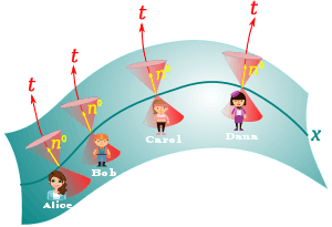
These properties can be used to construct synchronous frame in any spacetime (Fig. 2). To this end, choose some spacelike hypersurface as an origin, such that has in every point a normal along the time line (lies inside the light cone with an apex in that point); all interval elements on this hypersurface are space-like. Then draw a family of geodesics normal to this hypersurface. Choose these lines as time coordinate lines and define the time coordinate t as the length s of the geodesic measured with a beginning at the hypersurface; the result is a synchronous frame.

An analytic transformation to synchronous frame can be done with the use of the Hamilton–Jacobi equation. The principle of this method is based on the fact that particle trajectories in gravitational fields are geodesics. The Hamilton–Jacobi equation for a particle (whose mass is set equal to unity) in a gravitational field is

$g^{ik}{\frac {\partial S}{\partial x^{i}}}{\frac {\partial S}{\partial x^{k}}}=1,$

(eq. 18a)

where S is the action. Its complete integral has the form:

$S=f\left(\xi ^{\alpha },x^{i}\right)+A\left(\xi ^{\alpha }\right),$

(eq. 18b)

where f is a function of the four coordinates xⁱ and the three parameters ξ^α; the constant A is treated as an arbitrary function of the three ξ^α. With such a representation for S the equations for the trajectory of the particle can be obtained by equating the derivatives ∂S/∂ξ^α to zero, i.e.

${\frac {\partial f}{\partial \xi ^{\alpha }}}=-{\frac {\partial A}{\partial \xi ^{\alpha }}}.$

(eq. 18c)

For each set of assigned values of the parameters ξ^α, the right sides of equations 18a-18c have definite constant values, and the world line determined by these equations is one of the possible trajectories of the particle. Choosing the quantities ξ^α, which are constant along the trajectory, as new space coordinates, and the quantity S as the new time coordinate, one obtains a synchronous reference system; the transformation from the old coordinates to the new ones is given by equations 18b-18c. In fact, it is guaranteed that for such a transformation the time lines will be geodesics and will be normal to the hypersurfaces S = const. The latter point is obvious from the mechanical analogy: the four-vector ∂S/∂xⁱ which is normal to the hypersurface coincides in mechanics with the four-momentum of the particle, and therefore coincides in direction with its four-velocity uⁱ i.e. with the four-vector tangent to the trajectory. Finally the condition g₀₀ = 1 is obviously satisfied, since the derivative −dS/ds of the action along the trajectory is the mass of the particle, which was set equal to 1; therefore |dS/ds| = 1.

The gauge conditions eq. 15 do not fix the coordinate system completely and therefore are not a fixed gauge, as the spacelike hypersurface at $t=0$ can be chosen arbitrarily. One still have the freedom of performing some coordinate transformations containing four arbitrary functions depending on the three spatial variables x^α, which are easily worked out in infinitesimal form:

$x^{i}={\acute {x}}^{i}+\xi ^{i}({\acute {x}}).$

(eq. 18)

Here, the collections of the four old coordinates (t, x^α) and four new coordinates $({\acute {t}},{\acute {x}}^{\alpha })$ are denoted by the symbols x and ${\acute {x}}$ , respectively. The functions $\xi ^{i}({\acute {x}})$ together with their first derivatives are infinitesimally small quantities. After such a transformation, the four-dimensional interval takes the form:

$ds^{2}=g_{ik}(x)dx^{i}dx^{k}=g_{ik}^{(new)}({\acute {x}})d{\acute {x}}^{i}d{\acute {x}}^{k},$

(eq. 19)

where

$g_{ik}^{(new)}({\acute {x}})=g_{ik}({\acute {x}})+g_{il}({\acute {x}}){\frac {\partial \xi ^{l}({\acute {x}})}{\partial {\acute {x}}^{k}}}+g_{kl}({\acute {x}}){\frac {\partial \xi ^{l}({\acute {x}})}{\partial {\acute {x}}^{i}}}+{\frac {\partial g_{ik}({\acute {x}})}{\partial {\acute {x}}^{l}}}\xi ^{l}({\acute {x}}).$

(eq. 20)

In the last formula, the $g_{ik}({\acute {x}})$ are the same functions g_ik(x) in which x should simply be replaced by ${\acute {x}}$ . If one wishes to preserve the gauge eq. 15 also for the new metric tensor $g_{ik}^{(new)}({\acute {x}})$ in the new coordinates ${\acute {x}}$ , it is necessary to impose the following restrictions on the functions $\xi ^{i}({\acute {x}})$ :

${\frac {\partial \xi ^{0}({\acute {x}})}{\partial {\acute {x}}}}=0,\quad g_{\alpha \beta }({\acute {x}}){\frac {\partial \xi ^{\beta }({\acute {x}})}{\partial {\acute {t}}}}-{\frac {\partial \xi ^{0}({\acute {x}})}{\partial {\acute {x}}^{\alpha }}}=0.$

(eq. 21)

The solutions of these equations are:

$\xi ^{0}=f^{0}\left({\acute {x}}^{1},{\acute {x}}^{2},{\acute {x}}^{3}\right),\quad \xi ^{\alpha }=\int {g^{\alpha \beta }({\acute {x}}){\frac {\partial f^{0}\left({\acute {x}}^{1},{\acute {x}}^{2},{\acute {x}}^{3}\right)}{\partial {\acute {x}}^{\beta }}}d{\acute {x}}^{0}}+f^{\alpha }\left({\acute {x}}^{1},{\acute {x}}^{2},{\acute {x}}^{3}\right),$

(eq. 22)

where f⁰ and f^α are four arbitrary functions depending only on the spatial coordinates ${\acute {x}}^{\alpha }$ .

For a more elementary geometrical explanation, consider Fig. 2. First, the synchronous time line ξ⁰ = t can be chosen arbitrarily (Bob's, Carol's, Dana's or any of an infinitely many observers). This makes one arbitrarily chosen function: $\xi ^{0}=f^{0}\left({\acute {x}}^{1},{\acute {x}}^{2},{\acute {x}}^{3}\right)$ . Second, the initial hypersurface can be chosen in infinitely many ways. Each of these choices changes three functions: one function for each of the three spatial coordinates $\xi ^{\alpha }=f^{\alpha }\left({\acute {x}}^{1},{\acute {x}}^{2},{\acute {x}}^{3}\right)$ . Altogether, four (= 1 + 3) functions are arbitrary.

When discussing general solutions g_αβ of the field equations in synchronous gauges, it is necessary to keep in mind that the gravitational potentials g_αβ contain, among all possible arbitrary functional parameters present in them, four arbitrary functions of 3-space just representing the gauge freedom and therefore of no direct physical significance.

Another problem with the reference system is that caustics can occur which cause the gauge choice to break down. These problems have caused some difficulties doing cosmological perturbation theory in this system, but the problems are now well understood. Synchronous coordinates are generally considered the most efficient reference system for doing calculations, and are used in many modern cosmology codes, such as CMBFAST. They are also useful for solving theoretical problems in which a spacelike hypersurface needs to be fixed, as with spacelike singularities.

Einstein equations in synchronous frame

Introduction of a synchronous frame allows one to separate the operations of space and time differentiation in the Einstein field equations. To make them more concise, the notation

$\varkappa _{\alpha \beta }={\frac {\partial \gamma _{\alpha \beta }}{\partial t}}$

(eq. 23)

is introduced for the time derivatives of the three-dimensional metric tensor; these quantities also form a three-dimensional tensor. In the synchronous frame $\varkappa _{\alpha \beta }$ is proportional to the second fundamental form (shape tensor). All operations of shifting indices and covariant differentiation of the tensor $\varkappa _{\alpha \beta }$ are done in three-dimensional space with the metric γ_αβ. This does not apply to operations of shifting indices in the space components of the four-tensors R_ik, T_ik. Thus T_α^β must be understood to be g^βγT_γα + g^β0T_0α, which reduces to g^βγT_γα and differs in sign from γ^βγT_γα. The sum $\varkappa _{\alpha }^{\alpha }$ is the logarithmic derivative of the determinant γ ≡ |γ_αβ| = − g:

$\varkappa _{\alpha }^{\alpha }=\gamma ^{\alpha \beta }{\frac {\partial \gamma _{\alpha \beta }}{\partial t}}={\frac {\partial }{\partial t}}\ln {(\gamma )}.$

(eq. 24)

Then for the complete set of Christoffel symbols $\Gamma _{kl}^{i}$ one obtains:

$\Gamma _{00}^{0}=\Gamma _{00}^{\alpha }=\Gamma _{0\alpha }^{0}=0,\quad \Gamma _{\alpha \beta }^{0}={\frac {1}{2}}\varkappa _{\alpha \beta },\quad \Gamma _{0\beta }^{\alpha }={\frac {1}{2}}\varkappa _{\beta }^{\alpha },\quad \Gamma _{\alpha \beta }^{\gamma }=\lambda _{\alpha \beta }^{\gamma }$

(eq. 25)

where $\lambda _{\alpha \beta }^{\gamma }$ are the three-dimensional Christoffel symbols constructed from γ_αβ:

$\lambda _{\alpha \beta }^{\gamma }={\frac {1}{2}}\gamma ^{\gamma \mu }\left(\gamma _{\mu \alpha ,\beta }+\gamma _{\mu \beta ,\beta }-\gamma _{\alpha \beta ,\mu }\right),$

(eq. 26)

where the comma denotes partial derivative by the respective coordinate.

With the Christoffel symbols eq. 25, the components Rⁱ_k = g^ilR_lk of the Ricci tensor can be written in the form:

$R_{0}^{0}=-{\frac {1}{2}}{\dot {\varkappa }}-{\frac {1}{4}}\varkappa _{\alpha }^{\beta }\varkappa _{\beta }^{\alpha },$

(eq. 27)

$R_{\alpha }^{0}={\frac {1}{2}}\left(\varkappa _{\alpha ;\beta }^{\beta }-\varkappa _{,\alpha }\right),$

(eq. 28)

$R_{\alpha }^{\beta }=-{\frac {1}{2{\sqrt {\gamma }}}}{\dot {\left({\sqrt {\gamma }}\varkappa _{\alpha }^{\beta }\right)}}-P_{\alpha }^{\beta }.$

(eq. 29)

Dots on top denote time differentiation, semicolons (";") denote covariant differentiation which in this case is performed with respect to the three-dimensional metric γ_αβ with three-dimensional Christoffel symbols $\lambda _{\alpha \beta }^{\gamma }$ , $\varkappa \equiv \varkappa _{\alpha }^{\alpha }$ , and P_α^β is a three-dimensional Ricci tensor constructed from $\lambda _{\alpha \beta }^{\gamma }$ :

$P_{\alpha }^{\beta }=\gamma ^{\beta \gamma }P_{\gamma \alpha },\quad P_{\alpha \beta }=\lambda _{\alpha \beta ,\gamma }^{\gamma }-\lambda _{\gamma \alpha ,\beta }^{\gamma }+\lambda _{\alpha \beta }^{\gamma }\lambda _{\gamma \mu }^{\mu }-\lambda _{\alpha \mu }^{\gamma }\lambda _{\beta \gamma }^{\mu }.$

(eq. 30)

It follows from eq. 27–29 that the Einstein equations $R_{i}^{k}=8\pi k\left(T_{i}^{k}-{\frac {1}{2}}\delta _{i}^{k}T\right)$ (with the components of the energy-momentum tensor T₀⁰ = −T₀₀, T_α⁰ = −T_0α, T_α^β = γ^βγT_γα) become in a synchronous coordinate system:

$R_{0}^{0}=-{\frac {1}{2}}{\dot {\varkappa }}-{\frac {1}{4}}\varkappa _{\alpha }^{\beta }\varkappa _{\beta }^{\alpha }=8\pi k\left(T_{0}^{0}-{\frac {1}{2}}T\right),$

(eq. 31)

$R_{\alpha }^{0}={\frac {1}{2}}\left(\varkappa _{\alpha ;\beta }^{\beta }-\varkappa _{,\alpha }\right)=8\pi kT_{\alpha }^{0},$

(eq. 32)

$R_{\alpha }^{\beta }=-{\frac {1}{2{\sqrt {\gamma }}}}{\dot {\left({\sqrt {\gamma }}\varkappa _{\alpha }^{\beta }\right)}}-P_{\alpha }^{\beta }=8\pi k\left(T_{\alpha }^{\beta }-{\frac {1}{2}}\delta _{\alpha }^{\beta }T\right).$

(eq. 33)

A characteristic feature of synchronous reference systems is that they are not stationary: the gravitational field cannot be constant in such a system. In a constant field $\varkappa _{\alpha \beta }$ would become zero. But in the presence of matter the disappearance of all $\varkappa _{\alpha \beta }$ would contradict eq. 31 (which has a right side different from zero). In empty space from eq. 33 follows that all P_αβ, and with them all the components of the three-dimensional curvature tensor P_αβγδ (Riemann tensor) vanish, i.e. the field vanishes entirely (in a synchronous system with a Euclidean spatial metric the space-time is flat).

At the same time the matter filling the space cannot in general be at rest relative to the synchronous reference frame. This is obvious from the fact that particles of matter within which there are pressures generally move along lines that are not geodesics; the world line of a particle at rest is a time line, and thus is a geodesic in the synchronous reference system. An exception is the case of dust (p = 0). Here the particles interacting with one another will move along geodesic lines; consequently, in this case the condition for a synchronous reference system does not contradict the condition that it be comoving with the matter. Even in this case, in order to be able to choose a synchronously comoving system of reference, it is still necessary that the matter move without rotation. In the comoving system the contravariant components of the velocity are u⁰ = 1, u^α = 0. If the reference system is also synchronous, the covariant components must satisfy u₀ = 1, u_α = 0, so that its four-dimensional curl must vanish:

u_{i;k}-u_{k;i}\equiv {\frac {\partial u_{i}}{\partial x^{k}}}-{\frac {\partial u_{k}}{\partial x^{i}}}=0.

But this tensor equation must then also be valid in any other reference frame. Thus, in a synchronous but not comoving system the condition curl v = 0 for the three-dimensional velocity v is additionally needed. For other equations of state a similar situation can occur only in special cases when the pressure gradient vanishes in all or in certain directions.

References

Landau, Lev D.; Lifshitz, Evgeny M. (1988), Classical Theory of Fields (7th Russian ed.), Moscow: Nauka, ISBN 5-02-014420-7 Vol. 2 of the Course of Theoretical Physics.
Carroll, Sean M. (2004). Spacetime and Geometry: An Introduction to General Relativity. San Francisco: Addison-Wesley. ISBN 0-8053-8732-3. . See section 7.2.
C.-P. Ma & E. Bertschinger (1995). "Cosmological perturbation theory in the synchronous and conformal Newtonian gauges". Astrophys. J. 455: 7–25. arXiv:astro-ph/9506072. Bibcode:1995ApJ...455....7M. doi:10.1086/176550.
Landau, L.D. and Lifshitz, E.M. (1972). The Classical Theory of Fields. England: Elsevier Butterworth Heinemann. ISBN 0-7506-2768-9. . See section 97.

This article is issued from Wikipedia. The text is licensed under Creative Commons - Attribution - Sharealike. Additional terms may apply for the media files.