Simpson's rule

Simpson's rule can be derived by approximating the integrand f (x) (in blue) by the quadratic interpolant P(x) (in red).

An animation showing how Simpson's rule approximation improves with more strips.

In numerical analysis, Simpson's rule is a method for numerical integration, the numerical approximation of definite integrals. Specifically, it is the following approximation for $n$ equally spaced subdivisions (where $n$ is even): (General Form)

\int _{a}^{b}f(x)\,dx\approx {\tfrac {\Delta x}{3}}\left(f(x_{0})+4f(x_{1})+2f(x_{2})+4f(x_{3})+2f(x_{4})+\cdots +4f(x_{n-1})+f(x_{n})\right)

,

where $\Delta x={\frac {b-a}{n}}$ and $x_{i}=a+i\Delta x$ .

For unequally spaced points, see Cartwright.^[1]

Simpson's rule also corresponds to the three-point Newton-Cotes quadrature rule.

In English, the method is credited to the mathematician Thomas Simpson (1710–1761) of Leicestershire, England. However, Johannes Kepler used similar formulas over 100 years prior, and for this reason the method is sometimes called Kepler's rule, or Keplersche Fassregel (Kepler's barrel rule) in German.

Derivation

Simpson's rule can be derived in various ways.

Quadratic interpolation

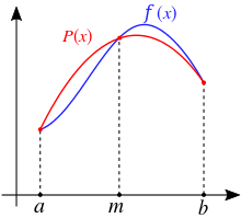
One derivation replaces the integrand $f(x)$ by the quadratic polynomial (i.e. parabola) $P(x)$ which takes the same values as $f(x)$ at the end points a and b and the midpoint m = (a + b) / 2. One can use Lagrange polynomial interpolation to find an expression for this polynomial,

P(x)=f(a){\tfrac {(x-m)(x-b)}{(a-m)(a-b)}}+f(m){\tfrac {(x-a)(x-b)}{(m-a)(m-b)}}+f(b){\tfrac {(x-a)(x-m)}{(b-a)(b-m)}}.

Using integration by substitution one can show that^[2]

\int _{a}^{b}P(x)\,dx={\tfrac {b-a}{6}}\left[f(a)+4f\left({\tfrac {a+b}{2}}\right)+f(b)\right].

Introducing the step size $h=(b-a)/2$ this is also commonly written as

\int _{a}^{b}P(x)\,dx={\tfrac {h}{3}}\left[f(a)+4f\left({\tfrac {a+b}{2}}\right)+f(b)\right].

Because of the $1/3$ factor Simspon's rule is also referred to as Simpson's 1/3 rule (see below for generalization).

The calculation above can be simplified if one observes that (by scaling) there is no loss of generality in assuming that $a=-1$ and $b=1$ .

Averaging the midpoint and the trapezoidal rules

Another derivation constructs Simpson's rule from two simpler approximations: the midpoint rule

M=(b-a)f\left({\tfrac {a+b}{2}}\right)

and the trapezoidal rule

T={\tfrac {1}{2}}(b-a)(f(a)+f(b)).

The errors in these approximations are

{\tfrac {1}{24}}(b-a)^{3}f''(a)+O((b-a)^{4})\quad {\text{and}}\quad -{\tfrac {1}{12}}(b-a)^{3}f''(a)+O((b-a)^{4}),

respectively, where $O((b-a)^{4})$ denotes a term asymptotically proportional to $(b-a)^{4}$ . The two $O((b-a)^{4})$ terms are not equal; see Big O notation for more details. It follows from the above formulas for the errors of the midpoint and trapezoidal rule that the leading error term vanishes if we take the weighted average

{\tfrac {2M+T}{3}}.

This weighted average is exactly Simpson's rule.

Using another approximation (for example, the trapezoidal rule with twice as many points), it is possible to take a suitable weighted average and eliminate another error term. This is Romberg's method.

Undetermined coefficients

The third derivation starts from the ansatz

{\tfrac {1}{b-a}}\int _{{a}}^{{b}}f(x)\,dx\approx \alpha f(a)+\beta f\left({\tfrac {a+b}{2}}\right)+\gamma f(b).

The coefficients α, β and γ can be fixed by requiring that this approximation be exact for all quadratic polynomials. This yields Simpson's rule.

Error

The error in approximating an integral by Simpson's rule is

-{\tfrac {1}{90}}\left({\tfrac {b-a}{2}}\right)^{5}f^{(4)}(\xi ),

where $\xi$ is some number between $a$ and $b$ .^[3]

The error is asymptotically proportional to $(b-a)^{5}$ . However, the above derivations suggest an error proportional to $(b-a)^{4}$ . Simpson's rule gains an extra order because the points at which the integrand is evaluated are distributed symmetrically in the interval [a, b].

Since the error term is proportional to the fourth derivative of f at $\xi$ , this shows that Simpson's rule provides exact results for any polynomial f of degree three or less, since the fourth derivative of such a polynomial is zero at all points.

Composite Simpson's rule

If the interval of integration $[a,b]$ is in some sense "small", then Simpson's rule will provide an adequate approximation to the exact integral. By small, what we really mean is that the function being integrated is relatively smooth over the interval $[a,b]$ . For such a function, a smooth quadratic interpolant like the one used in Simpson's rule will give good results.

However, it is often the case that the function we are trying to integrate is not smooth over the interval. Typically, this means that either the function is highly oscillatory, or it lacks derivatives at certain points. In these cases, Simpson's rule may give very poor results. One common way of handling this problem is by breaking up the interval $[a,b]$ into a number of small subintervals. Simpson's rule is then applied to each subinterval, with the results being summed to produce an approximation for the integral over the entire interval. This sort of approach is termed the composite Simpson's rule.

Suppose that the interval $[a,b]$ is split up into $n$ subintervals, with $n$ an even number. Then, the composite Simpson's rule is given by

{\begin{aligned}\int _{a}^{b}f(x)\,dx&\approx {\frac {h}{3}}\sum _{j=1}^{n/2}{\bigg [}f(x_{2j-2})+4f(x_{2j-1})+f(x_{2j}){\bigg ]}\\{}&={\frac {h}{3}}{\bigg [}f(x_{0})+2\sum _{j=1}^{n-2}f(x_{2j})+4\sum _{j=1}^{n-1}f(x_{2j-1})+f(x_{n}){\bigg ]},\end{aligned}}

where $x_{j}=a+jh$ for $j=0,1,...,n-1,n$ with $h=(b-a)/n$ ; in particular, $x_{0}=a$ and $x_{n}=b$ . This composite rule with $n=2$ corresponds with the regular Simpson's Rule of the preceding section.

The error committed by the composite Simpson's rule is

-{\frac {h^{4}}{180}}(b-a)f^{(4)}(\xi ),

where $\xi$ is some number between $a$ and $b$ and $h=(b-a)/n$ is the "step length".^[4] The error is bounded (in absolute value) by

{\tfrac {h^{4}}{180}}(b-a)\max _{\xi \in [a,b]}|f^{(4)}(\xi )|.

This formulation splits the interval $[a,b]$ in subintervals of equal length. In practice, it is often advantageous to use subintervals of different lengths, and concentrate the efforts on the places where the integrand is less well-behaved. This leads to the adaptive Simpson's method.

Simpson's 3/8 rule

Simpson's 3/8 rule is another method for numerical integration proposed by Thomas Simpson. It is based upon a cubic interpolation rather than a quadratic interpolation. Simpson's 3/8 rule is as follows:

\int _{a}^{b}f(x)\,dx\approx {\tfrac {3h}{8}}\left[f(a)+3f\left({\tfrac {2a+b}{3}}\right)+3f\left({\tfrac {a+2b}{3}}\right)+f(b)\right]={\tfrac {(b-a)}{8}}\left[f(a)+3f\left({\tfrac {2a+b}{3}}\right)+3f\left({\tfrac {a+2b}{3}}\right)+f(b)\right],

where b − a = 3h. The error of this method is:

-{\tfrac {(b-a)^{5}}{6480}}f^{(4)}(\xi ),

where $\xi$ is some number between $a$ and $b$ . Thus, the 3/8 rule is about twice as accurate as the standard method, but it uses one more function value. A composite 3/8 rule also exists, similarly as above.^[5]

A further generalization of this concept for interpolation with arbitrary-degree polynomials are the Newton–Cotes formulas.

Composite Simpson's 3/8 rule

Dividing the interval $[a,b]$ into $n$ subintervals of length $h=(b-a)/n$ and introducing the nodes $x_i = a + ih$ we have

{\begin{aligned}\int _{a}^{b}f(x)\,dx&\approx {\tfrac {3h}{8}}\left[f(x_{0})+3f(x_{1})+3f(x_{2})+2f(x_{3})+3f(x_{4})+3f(x_{5})+2f(x_{6})+\cdots +f(x_{n})\right].\\&={\frac {3h}{8}}\left[f(x_{0})+3\sum _{i\neq 3k}^{n-1}f(x_{i})+2\sum _{j=1}^{n/3-1}f(x_{3j})+f(x_{n})\right]\qquad {\text{For:  }}k\in \mathbb {N} _{0}\end{aligned}}

While the remainder for the rule is shown as:

-{\frac {h^{4}}{80}}(b-a)f^{(4)}(\xi ),

^[6]

Note, we can only use this if $n$ is a multiple of three.

A simplified version of Simpson's rules is used in naval architecture. The 3/8th rule is also called Simpson's second rule.

Alternative extended Simpson's rule

This is another formulation of a composite Simpson's rule: instead of applying Simpson's rule to disjoint segments of the integral to be approximated, Simpson's rule is applied to overlapping segments, yielding:^[7]

\int _{a}^{b}f(x)\,dx\approx {\tfrac {h}{48}}{\bigg [}17f(x_{0})+59f(x_{1})+43f(x_{2})+49f(x_{3})+48\sum _{{i=4}}^{{n-4}}f(x_{i})+49f(x_{{n-3}})+43f(x_{{n-2}})+59f(x_{{n-1}})+17f(x_{n}){\bigg ]}.

The formula above is obtained by combining the original composite Simpson's rule with the one consisting of using Simpson's 3/8 rule in the extreme subintervals and the standard 3-point rule in the remaining subintervals. The result is then obtained by taking the mean of the two formulas.

Simpson's rules in the case of narrow peaks

In the task of estimation of full area of narrow peak-like functions, Simpson's rules are much less efficient than trapezoidal rule. Namely, composite Simpson's 1/3 rule requires 1.8 times more points to achieve the same accuracy^[8] as trapezoidal rule. Composite Simpson's 3/8 rule is even less accurate. Integral by Simpson's 1/3 rule can be represented as a sum of 2/3 of integral by trapezoidal rule with step h and 1/3 of integral by rectangle rule with step 2h. No wonder that error of the sum corresponds lo less accurate term. Averaging of Simpson's 1/3 rule composite sums with properly shifted frames produces following rules:

$\int _{a}^{b}f(x)\,dx\approx {\tfrac {h}{24}}{\bigg [}-f(x_{0})+12f(x_{1})+23f(x_{2})+24\sum _{i=2}^{n-2}f(x_{i})+23f(x_{n-1})+12f(x_{n})-f(x_{n+1}){\bigg ]}$

where two points outside of integrated region are exploited and

$\int _{a}^{b}f(x)\,dx\approx {\tfrac {h}{24}}{\bigg [}9f(x_{1})+28f(x_{2})+23f(x_{3})+24\sum _{i=3}^{n-3}f(x_{i})+23f(x_{n-2})+28f(x_{n-1})+9f(x_{n}){\bigg ]}$

Those rules are very much similar to Press's alternative extended Simpson's rule. Coefficients within the major part of the region being integrated equal one, differences are only at the edges. These three rules can be associated with Euler-MacLaurin formula with the first derivative term and named Euler-MacLaurin integration rules^[8]. They differ only in the way, how the first derivative at the region end is calculated.

Notes

↑ Cartwright, Kenneth V. (2016). "Simpson's Rule Integration with MS Excel and Irregularly-spaced Data" (PDF). Journal of Mathematical Science and Mathematics Education. 11 (2): 34–42.
↑ Atkinson, p. 256; Süli and Mayers, §7.2
↑ Atkinson, equation (5.1.15); Süli and Mayers, Theorem 7.2
↑ Atkinson, pp. 257+258; Süli and Mayers, §7.5
↑ Matthews (2004)
↑ Matthews (2004)
↑ Press (1989), p. 122
1 2 Kalambet, Yuri; Kozmin, Yuri; Samokhin, Andrey (2018). "Comparison of integration rules in the case of very narrow chromatographic peaks". Chemometrics and Intelligent Laboratory Systems. 179: 22–30. doi:10.1016/j.chemolab.2018.06.001. ISSN 0169-7439.

References

Atkinson, Kendall E. (1989). An Introduction to Numerical Analysis (2nd ed.). John Wiley & Sons. ISBN 0-471-50023-2.
Burden, Richard L.; Faires, J. Douglas (2000). Numerical Analysis (7th ed.). Brooks/Cole. ISBN 0-534-38216-9.
Pate, McCall (1918). The naval artificer's manual: (The naval artificer's handbook revised) text, questions and general information for deck. United States. Bureau of Reconstruction and Repair. p. 198.
Matthews, John H. (2004). "Simpson's 3/8 Rule for Numerical Integration". Numerical Analysis - Numerical Methods Project. California State University, Fullerton. Archived from the original on 4 December 2008. Retrieved 11 November 2008.
Press, William H.; Flannery, Brian P.; Vetterling, William T.; Teukolsky, Saul A. (1989). Numerical Recipes in Pascal: The Art of Scientific Computing. Cambridge University Press. ISBN 0-521-37516-9.
Süli, Endre; Mayers, David (2003). An Introduction to Numerical Analysis. Cambridge University Press. ISBN 0-521-00794-1.
Kaw, Autar; Kalu, Egwu; Nguyen, Duc (2008). "Numerical Methods with Applications".
Weisstein, Eric W. (2010). "Newton-Cotes Formulas". MathWorld--A Wolfram Web Resource. MathWorld. Retrieved 2 August 2010.

External links

Hazewinkel, Michiel, ed. (2001) [1994], "Simpson formula", Encyclopedia of Mathematics, Springer Science+Business Media B.V. / Kluwer Academic Publishers, ISBN 978-1-55608-010-4
Weisstein, Eric W. "Simpson's Rule". MathWorld.
Application of Simpson's Rule — Earthwork Excavation (Note: The formula described in this page is correct but there are errors in the calculation which should give a result of 569m3 and not 623m3 as stated)
Simpson's 1/3rd rule of integration — Notes, PPT, Mathcad, Matlab, Mathematica, Maple at Numerical Methods for STEM undergraduate
A detailed description of a computer implementation is described by Dorai Sitaram in Teach Yourself Scheme in Fixnum Days, Appendix C

This article incorporates material from Code for Simpson's rule on PlanetMath, which is licensed under the Creative Commons Attribution/Share-Alike License.

This article is issued from Wikipedia. The text is licensed under Creative Commons - Attribution - Sharealike. Additional terms may apply for the media files.

[1] Cartwright, Kenneth V. (2016). "Simpson's Rule Integration with MS Excel and Irregularly-spaced Data" (PDF). Journal of Mathematical Science and Mathematics Education. 11 (2): 34–42.

[2] Atkinson, p. 256; Süli and Mayers, §7.2

[3] Atkinson, equation (5.1.15); Süli and Mayers, Theorem 7.2

[4] Atkinson, pp. 257+258; Süli and Mayers, §7.5

[5] Matthews (2004)

[6] Matthews (2004)

[7] Press (1989), p. 122

[:0-8] 1 2 Kalambet, Yuri; Kozmin, Yuri; Samokhin, Andrey (2018). "Comparison of integration rules in the case of very narrow chromatographic peaks". Chemometrics and Intelligent Laboratory Systems. 179: 22–30. doi:10.1016/j.chemolab.2018.06.001. ISSN 0169-7439.