''p''-value
In statistical hypothesis testing, the p-value or probability value or asymptotic significance is the probability for a given statistical model that, when the null hypothesis is true, the statistical summary (such as the sample mean difference between two compared groups) would be greater or equal to the actual observed results.[1] The use of p-values in statistical hypothesis testing is common in many fields of research[2] such as physics, economics, finance, political science, psychology,[3] biology, criminal justice, criminology, and sociology.[4] Their misuse has been a matter of considerable controversy.
Italicisation, capitalisation and hyphenation of the term varies. For example, AMA style uses "P value," APA style uses "p value," and the American Statistical Association uses "p-value."[5]
Basic concepts
The p-value is used in the context of null hypothesis testing in order to quantify the idea of statistical significance of evidence.[lower-alpha 1] Null hypothesis testing is a reductio ad absurdum argument adapted to statistics. In essence, a claim is assumed valid if its counter-claim is improbable.
As such, the only hypothesis that needs to be specified in this test and which embodies the counter-claim is referred to as the null hypothesis (that is, the hypothesis to be nullified). A result is said to be statistically significant if it allows us to reject the null hypothesis. That is, as per the reductio ad absurdum reasoning, the statistically significant result should be highly improbable if the null hypothesis is assumed to be true. The rejection of the null hypothesis implies that the correct hypothesis lies in the logical complement of the null hypothesis. However, unless there is a single alternative to the null hypothesis, the rejection of null hypothesis does not tell us which of the alternatives might be the correct one.
As a general example, if a null hypothesis is assumed to follow the standard normal distribution N(0,1), then the rejection of this null hypothesis can either mean (i) the mean is not zero, or (ii) the variance is not unity, or (iii) the distribution is not normal, depending on the type of test performed. However, supposing we manage to reject the zero mean hypothesis, even if we know the distribution is normal and variance is unity, the null hypothesis test does not tell us which non-zero value we should adopt as the new mean.
If is a random variable representing the observed data and is the statistical hypothesis under consideration, then the notion of statistical significance can be naively quantified by the conditional probability , which gives the likelihood of the observation if the hypothesis is assumed to be correct. However, if is a continuous random variable and an instance is observed, Thus, this naive definition is inadequate and needs to be changed so as to accommodate the continuous random variables.


Nonetheless, it helps to clarify that p-values should not be confused with probability on hypothesis (as is done in Bayesian hypothesis testing) such as the probability of the hypothesis given the data, or the probability of the hypothesis being true, or the probability of observing the given data.


Definition and interpretation
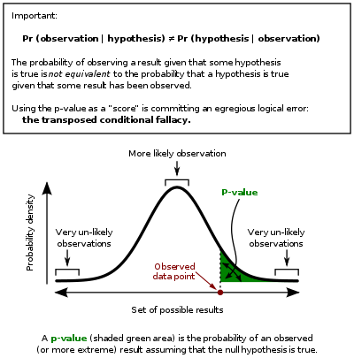
The p-value is defined as the probability, under the null hypothesis, here simply denoted by (but is often denoted , as opposed to , which is sometimes used to represent the alternative hypothesis), of obtaining a result equal to or more extreme than what was actually observed. Depending on how it is looked at, the "more extreme than what was actually observed" can mean (right-tail event) or (left-tail event) or the "smaller" of and (double-tailed event). Thus, the p-value is given by


- for right tail event,
- for left tail event,
- for double tail event.


The smaller the p-value, the higher the significance because it tells the investigator that the hypothesis under consideration may not adequately explain the observation. The null hypothesis is rejected if any of these probabilities is less than or equal to a small, fixed but arbitrarily pre-defined threshold value , which is referred to as the level of significance. Unlike the p-value, the level is not derived from any observational data and does not depend on the underlying hypothesis; the value of is instead set by the researcher before examining the data. The setting of is arbitrary. By convention, is commonly set to 0.05, 0.01, 0.005, or 0.001.

Since the value of that defines the left tail or right tail event is a random variable, this makes the p-value a function of and a random variable in itself; under the null hypothesis, the p-value is defined uniformly over interval, assuming is continuous. Thus, the p-value is not fixed. This implies that p-value cannot be given a frequency counting interpretation since the probability has to be fixed for the frequency counting interpretation to hold. In other words, if the same test is repeated independently bearing upon the same overall null hypothesis, it will yield different p-values at every repetition. Nevertheless, these different p-values can be combined using Fisher's combined probability test. It should further be noted that an instantiation of this random p-value can still be given a frequency counting interpretation with respect to the number of observations taken during a given test, as per the definition, as the percentage of observations more extreme than the one observed under the assumption that the null hypothesis is true.
![[0,1]](../I/m/738f7d23bb2d9642bab520020873cccbef49768d.svg)
Misconceptions
There is widespread agreement that p-values are often misused and misinterpreted.[1][6][7] One practice that has been particularly criticized is accepting the alternative hypothesis for any p-value nominally less than .05 without other supporting evidence. Although p-values are helpful in assessing how incompatible the data are with a specified statistical model, contextual factors must also be considered, such as "the design of a study, the quality of the measurements, the external evidence for the phenomenon under study, and the validity of assumptions that underlie the data analysis".[1] Another concern is that the p-value is often misunderstood as being the probability that the null hypothesis is true.[1][8] Some statisticians have proposed replacing p-values with alternative measures of evidence,[1] such as confidence intervals,[9][10] likelihood ratios,[11][12] or Bayes factors,[13][14][15] but there is heated debate on the feasibility of these alternatives.[16][17] Others have suggested to remove fixed significance thresholds and to interpret p-values as continuous indices of the strength of evidence against the null hypothesis.[18][19]
Usage
The p-value is widely used in statistical hypothesis testing, specifically in null hypothesis significance testing. In this method, as part of experimental design, before performing the experiment, one first chooses a model (the null hypothesis) and a threshold value for p, called the significance level of the test, traditionally 5% or 1% [20] and denoted as α. If the p-value is less than the chosen significance level (α), that suggests that the observed data is sufficiently inconsistent with the null hypothesis that the null hypothesis may be rejected. However, that does not prove that the tested hypothesis is true. When the p-value is calculated correctly, this test guarantees that the type I error rate is at most α. For typical analysis, using the standard α = 0.05 cutoff, the null hypothesis is rejected when p < .05 and not rejected when p > .05. The p-value does not, in itself, support reasoning about the probabilities of hypotheses but is only a tool for deciding whether to reject the null hypothesis.
Calculation
Usually, is a test statistic, rather than any of the actual observations. A test statistic is the output of a scalar function of all the observations. This statistic provides a single number, such as the average or the correlation coefficient, that summarizes the characteristics of the data, in a way relevant to a particular inquiry. As such, the test statistic follows a distribution determined by the function used to define that test statistic and the distribution of the input observational data.
For the important case in which the data are hypothesized to follow the normal distribution, depending on the nature of the test statistic and thus the underlying hypothesis of the test statistic, different null hypothesis tests have been developed. Some such tests are z-test for normal distribution, t-test for Student's t-distribution, f-test for f-distribution. When the data do not follow a normal distribution, it can still be possible to approximate the distribution of these test statistics by a normal distribution by invoking the central limit theorem for large samples, as in the case of Pearson's chi-squared test.
Thus computing a p-value requires a null hypothesis, a test statistic (together with deciding whether the researcher is performing a one-tailed test or a two-tailed test), and data. Even though computing the test statistic on given data may be easy, computing the sampling distribution under the null hypothesis, and then computing its cumulative distribution function (CDF) is often a difficult problem. Today, this computation is done using statistical software, often via numeric methods (rather than exact formulae), but, in the early and mid 20th century, this was instead done via tables of values, and one interpolated or extrapolated p-values from these discrete values. Rather than using a table of p-values, Fisher instead inverted the CDF, publishing a list of values of the test statistic for given fixed p-values; this corresponds to computing the quantile function (inverse CDF).
Distribution
When the null hypothesis is true, if it takes the form , and the underlying random variable is continuous, then the probability distribution of the p-value is uniform on the interval [0,1]. By contrast, if the alternative hypothesis is true, the distribution is dependent on sample size and the true value of the parameter being studied.[2][21]

The distribution of p-values for a group of studies is called a p-curve.[22] The curve is affected by four factors: the proportion of studies that examined false null hypotheses, the power of the studies that investigated false null hypotheses, the alpha levels, and publication bias.[23] A p-curve can be used to assess the reliability of scientific literature, such as by detecting publication bias or p-hacking.[22][24]
Examples
Here a few simple examples follow, each illustrating a potential pitfall.
One roll of a pair of dice
Suppose a researcher rolls a pair of dice once and assumes a null hypothesis that the dice are fair, not loaded or weighted toward any specific number/roll/result; uniform. The test statistic is "the sum of the rolled numbers" and is one-tailed. The researcher rolls the dice and observes that both dice show 6, yielding a test statistic of 12. The p-value of this outcome is 1/36 (because under the assumption of the null hypothesis, the test statistic is uniformly distributed) or about 0.028 (the highest test statistic out of 6×6 = 36 possible outcomes). If the researcher assumed a significance level of 0.05, this result would be deemed significant and the hypothesis that the dice are fair would be rejected.
In this case, a single roll provides a very weak basis (that is, insufficient data) to draw a meaningful conclusion about the dice. This illustrates the danger with blindly applying p-value without considering the experiment design.
Five heads in a row
Suppose a researcher flips a coin five times in a row and assumes a null hypothesis that the coin is fair. The test statistic of "total number of heads" can be one-tailed or two-tailed: a one-tailed test corresponds to seeing if the coin is biased towards heads, but a two-tailed test corresponds to seeing if the coin is biased either way. The researcher flips the coin five times and observes heads each time (HHHHH), yielding a test statistic of 5. In a one-tailed test, this is the upper extreme of all possible outcomes, and yields a p-value of (1/2)5 = 1/32 ≈ 0.03. If the researcher assumed a significance level of 0.05, this result would be deemed significant and the hypothesis that the coin is fair would be rejected. In a two-tailed test, a test statistic of zero heads (TTTTT) is just as extreme and thus the data of HHHHH would yield a p-value of 2×(1/2)5 = 1/16 ≈ 0.06, which is not significant at the 0.05 level.
This demonstrates that specifying a direction (on a symmetric test statistic) halves the p-value (increases the significance) and can mean the difference between data being considered significant or not.
Sample size dependence
Suppose a researcher flips a coin some arbitrary number of times (n) and assumes a null hypothesis that the coin is fair. The test statistic is the total number of heads and is a two-tailed test. Suppose the researcher observes heads for each flip, yielding a test statistic of n and a p-value of 2/2n. If the coin was flipped only 5 times, the p-value would be 2/32 = 0.0625, which is not significant at the 0.05 level. But if the coin was flipped 10 times, the p-value would be 2/1024 ≈ 0.002, which is significant at the 0.05 level.
In both cases the data suggest that the null hypothesis is false (that is, the coin is not fair somehow), but changing the sample size changes the p-value. In the first case, the sample size is not large enough to allow the null hypothesis to be rejected at the 0.05 level (in fact, the p-value can never be below 0.05 for the coin example).
This demonstrates that in interpreting p-values, one must also know the sample size, which complicates the analysis.
Alternating coin flips
Suppose a researcher flips a coin ten times and assumes a null hypothesis that the coin is fair. The test statistic is the total number of heads and is two-tailed. Suppose the researcher observes alternating heads and tails with every flip (HTHTHTHTHT). This yields a test statistic of 5 and a p-value of 1 (completely unexceptional), as that is the expected number of heads.
Suppose instead that the test statistic for this experiment was the "number of alternations" (that is, the number of times when H followed T or T followed H), which is one-tailed. That would yield a test statistic of 9, which is extreme and has a p-value of . That would be considered extremely significant, well beyond the 0.05 level. These data indicate that, in terms of one test statistic, the data set is extremely unlikely to have occurred by chance, but it does not suggest that the coin is biased towards heads or tails.

By the first test statistic, the data yield a high p-value, suggesting that the number of heads observed is not unlikely. By the second test statistic, the data yield a low p-value, suggesting that the pattern of flips observed is very, very unlikely. There is no "alternative hypothesis" (so only rejection of the null hypothesis is possible) and such data could have many causes. The data may instead be forged, or the coin may be flipped by a magician who intentionally alternated outcomes.
This example demonstrates that the p-value depends completely on the test statistic used and illustrates that p-values can only help researchers to reject a null hypothesis, not consider other hypotheses.
Coin flipping
As an example of a statistical test, an experiment is performed to determine whether a coin flip is fair (equal chance of landing heads or tails) or unfairly biased (one outcome being more likely than the other).
Suppose that the experimental results show the coin turning up heads 14 times out of 20 total flips. The null hypothesis is that the coin is fair, and the test statistic is the number of heads. If a right-tailed test is considered, the p-value of this result is the chance of a fair coin landing on heads at least 14 times out of 20 flips. That probability can be computed from binomial coefficients as
![{\begin{aligned}&\operatorname {Prob} (14{\text{ heads}})+\operatorname {Prob} (15{\text{ heads}})+\cdots +\operatorname {Prob} (20{\text{ heads}})\\&={\frac {1}{2^{20}}}\left[{\binom {20}{14}}+{\binom {20}{15}}+\cdots +{\binom {20}{20}}\right]={\frac {60,\!460}{1,\!048,\!576}}\approx 0.058\end{aligned}}](../I/m/881773374a766f7580f8defe2246c00be0723ea0.svg)
This probability is the p-value, considering only extreme results that favor heads. This is called a one-tailed test. However, the deviation can be in either direction, favoring either heads or tails. The two-tailed p-value, which considers deviations favoring either heads or tails, may instead be calculated. As the binomial distribution is symmetrical for a fair coin, the two-sided p-value is simply twice the above calculated single-sided p-value: the two-sided p-value is 0.115.
In the above example:
- Null hypothesis (H0): The coin is fair, with Prob(heads) = 0.5
- Test statistic: Number of heads
- Level of significance: 0.05
- Observation O: 14 heads out of 20 flips; and
- Two-tailed p-value of observation O given H0 = 2*min(Prob(no. of heads ≥ 14 heads), Prob(no. of heads ≤ 14 heads))= 2*min(0.058, 0.978) = 2*0.058 = 0.115.
Note that the Prob(no. of heads ≤ 14 heads) = 1 - Prob(no. of heads ≥ 14 heads) + Prob(no. of head = 14) = 1 - 0.058 + 0.036 = 0.978; however, symmetry of the binomial distribution makes it an unnecessary computation to find the smaller of the two probabilities. Here, the calculated p-value exceeds 0.05, so the observation is consistent with the null hypothesis, as it falls within the range of what would happen 95% of the time were the coin in fact fair. Hence, the null hypothesis at the 5% level is not rejected. Although the coin did not fall evenly, the deviation from the expected outcome is small enough to be consistent with chance.
However, had one more head been obtained, the resulting p-value (two-tailed) would have been 0.0414 (4.14%). The null hypothesis is rejected when a 5% cut-off is used.
History
.jpg)
Computations of p-values date back to the 1700s, where they were computed for the human sex ratio at birth, and used to compute statistical significance compared to the null hypothesis of equal probability of male and female births.[25] John Arbuthnot studied this question in 1710,[26][27][28][29] and examined birth records in London for each of the 82 years from 1629 to 1710. In every year, the number of males born in London exceeded the number of females. Considering more male or more female births as equally likely, the probability of the observed outcome is 0.582, or about 1 in 4,836,000,000,000,000,000,000,000; in modern terms, the p-value. This is vanishingly small, leading Arbuthnot that this was not due to chance, but to divine providence: "From whence it follows, that it is Art, not Chance, that governs." In modern terms, he rejected the null hypothesis of equally likely male and female births at the p = 1/282 significance level. This is and other work by Arbuthnot is credited as "… the first use of significance tests …"[30] the first example of reasoning about statistical significance,[31] and "… perhaps the first published report of a nonparametric test …",[27] specifically the sign test; see details at Sign test § History.
The same question was later addressed by Pierre-Simon Laplace, who instead used a parametric test, modeling the number of male births with a binomial distribution:[32]
In the 1770s Laplace considered the statistics of almost half a million births. The statistics showed an excess of boys compared to girls. He concluded by calculation of a p-value that the excess was a real, but unexplained, effect.
The p-value was first formally introduced by Karl Pearson, in his Pearson's chi-squared test,[33] using the chi-squared distribution and notated as capital P.[33] The p-values for the chi-squared distribution (for various values of χ2 and degrees of freedom), now notated as P, was calculated in (Elderton 1902), collected in (Pearson 1914, pp. xxxi–xxxiii, 26–28, Table XII).
The use of the p-value in statistics was popularized by Ronald Fisher,[34] and it plays a central role in his approach to the subject.[35] In his influential book Statistical Methods for Research Workers (1925), Fisher proposed the level p = 0.05, or a 1 in 20 chance of being exceeded by chance, as a limit for statistical significance, and applied this to a normal distribution (as a two-tailed test), thus yielding the rule of two standard deviations (on a normal distribution) for statistical significance (see 68–95–99.7 rule).[36][lower-alpha 2][37]
He then computed a table of values, similar to Elderton but, importantly, reversed the roles of χ2 and p. That is, rather than computing p for different values of χ2 (and degrees of freedom n), he computed values of χ2 that yield specified p-values, specifically 0.99, 0.98, 0.95, 0,90, 0.80, 0.70, 0.50, 0.30, 0.20, 0.10, 0.05, 0.02, and 0.01.[38] That allowed computed values of χ2 to be compared against cutoffs and encouraged the use of p-values (especially 0.05, 0.02, and 0.01) as cutoffs, instead of computing and reporting p-values themselves. The same type of tables were then compiled in (Fisher & Yates 1938), which cemented the approach.[37]
As an illustration of the application of p-values to the design and interpretation of experiments, in his following book The Design of Experiments (1935), Fisher presented the lady tasting tea experiment,[39] which is the archetypal example of the p-value.
To evaluate a lady's claim that she (Muriel Bristol) could distinguish by taste how tea is prepared (first adding the milk to the cup, then the tea, or first tea, then milk), she was sequentially presented with 8 cups: 4 prepared one way, 4 prepared the other, and asked to determine the preparation of each cup (knowing that there were 4 of each). In that case, the null hypothesis was that she had no special ability, the test was Fisher's exact test, and the p-value was so Fisher was willing to reject the null hypothesis (consider the outcome highly unlikely to be due to chance) if all were classified correctly. (In the actual experiment, Bristol correctly classified all 8 cups.)

Fisher reiterated the p = 0.05 threshold and explained its rationale, stating:[40]
It is usual and convenient for experimenters to take 5 per cent as a standard level of significance, in the sense that they are prepared to ignore all results which fail to reach this standard, and, by this means, to eliminate from further discussion the greater part of the fluctuations which chance causes have introduced into their experimental results.
He also applies this threshold to the design of experiments, noting that had only 6 cups been presented (3 of each), a perfect classification would have only yielded a p-value of which would not have met this level of significance.[40] Fisher also underlined the interpretation of p, as the long-run proportion of values at least as extreme as the data, assuming the null hypothesis is true.

In later editions, Fisher explicitly contrasted the use of the p-value for statistical inference in science with the Neyman–Pearson method, which he terms "Acceptance Procedures".[41] Fisher emphasizes that while fixed levels such as 5%, 2%, and 1% are convenient, the exact p-value can be used, and the strength of evidence can and will be revised with further experimentation. In contrast, decision procedures require a clear-cut decision, yielding an irreversible action, and the procedure is based on costs of error, which, he argues, are inapplicable to scientific research.
Related quantities
A closely related concept is the E-value,[42] which is the expected number of times in multiple testing that one expects to obtain a test statistic at least as extreme as the one that was actually observed if one assumes that the null hypothesis is true. The E-value is the product of the number of tests and the p-value.
See also
Notes
- ↑ Note that the statistical significance of a result does not imply that the result is scientifically significant as well.
- ↑ To be precise the p = 0.05 corresponds to about 1.96 standard deviations for a normal distribution (two-tailed test), and 2 standard deviations corresponds to about a 1 in 22 chance of being exceeded by chance, or p ≈ 0.045; Fisher notes these approximations.
References
- 1 2 3 4 5 Wasserstein, Ronald L.; Lazar, Nicole A. (7 March 2016). "The ASA's Statement on p-Values: Context, Process, and Purpose". The American Statistician. 70 (2): 129–133. doi:10.1080/00031305.2016.1154108. Retrieved 30 October 2016.
- 1 2 Bhattacharya, Bhaskar; Habtzghi, DeSale (2002). "Median of the p value under the alternative hypothesis". The American Statistician. American Statistical Association. 56 (3): 202–6. doi:10.1198/000313002146. Retrieved 19 February 2016.
- ↑ Wetzels, R.; Matzke, D.; Lee, M. D.; Rouder, J. N.; Iverson, G. J.; Wagenmakers, E. -J. (2011). "Statistical Evidence in Experimental Psychology: An Empirical Comparison Using 855 t Tests". Perspectives on Psychological Science. 6 (3): 291–298. doi:10.1177/1745691611406923.
- ↑ Babbie, E. (2007). The practice of social research 11th ed. Thomson Wadsworth: Belmont, California.
- ↑ http://magazine.amstat.org/wp-content/uploads/STATTKadmin/style%5B1%5D.pdf
- ↑ "Scientists Perturbed by Loss of Stat Tool to Sift Research Fudge from Fact". Scientific American. April 16, 2015.
- ↑ Goodman SN (1999). "Toward evidence-based medical statistics. 1: The P value fallacy". Annals of Internal Medicine. 130 (12): 995–1004. doi:10.7326/0003-4819-130-12-199906150-00008. PMID 10383371.
- ↑ Colquhoun, David (2014). "An investigation of the false discovery rate and the misinterpretation of p-values". Royal Society Open Science. 1: 140216. doi:10.1098/rsos.140216.
- ↑ Lee, Dong Kyu (7 March 2017). "Alternatives to P value: confidence interval and effect size". Korean Journal of Anesthesiology. 69 (6): 555–562. doi:10.4097/kjae.2016.69.6.555. ISSN 2005-6419. PMC 5133225. PMID 27924194.
- ↑ Ranstam, J. (August 2012). "Why the P-value culture is bad and confidence intervals a better alternative". Osteoarthritis and Cartilage. 20 (8): 805–808. doi:10.1016/j.joca.2012.04.001. Retrieved 7 March 2017.
- ↑ Perneger, Thomas V (12 May 2001). "Sifting the evidence: Likelihood ratios are alternatives to P values". BMJ: British Medical Journal. 322 (7295): 1184. ISSN 0959-8138. PMC 1120301. PMID 11379590.
- ↑ Royall, Richard. "The Likelihood Paradigm for Statistical Evidence". The Nature of Scientific Evidence. pp. 119–152. doi:10.7208/chicago/9780226789583.003.0005.
- ↑ Schimmack, Ulrich (30 April 2015). "Replacing p-values with Bayes-Factors: A Miracle Cure for the Replicability Crisis in Psychological Science". Replicability-Index. Retrieved 7 March 2017.
- ↑ Marden, John I. (December 2000). "Hypothesis Testing: From p Values to Bayes Factors". Journal of the American Statistical Association. 95 (452): 1316. doi:10.2307/2669779.
- ↑ Stern, Hal S. (16 February 2016). "A Test by Any Other Name: Values, Bayes Factors, and Statistical Inference". Multivariate Behavioral Research. 51 (1): 23–29. doi:10.1080/00273171.2015.1099032. PMC 4809350. PMID 26881954.
- ↑ Murtaugh, Paul A. (March 2014). "In defense of p-values". Ecology. 95 (3): 611–617. doi:10.1890/13-0590.1.
- ↑ Aschwanden, Christie (Mar 7, 2016). "Statisticians Found One Thing They Can Agree On: It's Time To Stop Misusing P-Values". FiveThirtyEight.
- ↑ Amrhein, Valentin; Korner-Nievergelt, Fränzi; Roth, Tobias (2017). "The earth is flat (p > 0.05): significance thresholds and the crisis of unreplicable research". PeerJ. 5: e3544. doi:10.7717/peerj.3544.
- ↑ Amrhein, Valentin; Greenland, Sander (2017). "Remove, rather than redefine, statistical significance". Nature Human Behaviour. 1: 0224. doi:10.1038/s41562-017-0224-0.
- ↑ Nuzzo, R. (2014). "Scientific method: Statistical errors". Nature. 506 (7487): 150–152. doi:10.1038/506150a.
- ↑ Hung, H.M.J.; O'Neill, R.T.; Bauer, P.; Kohne, K. (1997). "The behavior of the p-value when the alternative hypothesis is true". Biometrics. International Biometric Society. 53 (1): 11–22. doi:10.2307/2533093. JSTOR 2533093.
- 1 2 Head ML, Holman L, Lanfear R, Kahn AT, Jennions MD (2015). "The extent and consequences of p-hacking in science". PLoS Biol. 13 (3): e1002106. doi:10.1371/journal.pbio.1002106. PMC 4359000. PMID 25768323.
- ↑ Lakens D (2015). "What p-hacking really looks like: a comment on Masicampo and LaLande (2012)". Q J Exp Psychol (Hove). 68 (4): 829–32. doi:10.1080/17470218.2014.982664. PMID 25484109.
- ↑ Simonsohn U, Nelson LD, Simmons JP (2014). "p-Curve and Effect Size: Correcting for Publication Bias Using Only Significant Results". Perspect Psychol Sci. 9 (6): 666–81. doi:10.1177/1745691614553988. PMID 26186117.
- ↑ Brian, Éric; Jaisson, Marie (2007). "Physico-Theology and Mathematics (1710–1794)". The Descent of Human Sex Ratio at Birth. Springer Science & Business Media. pp. 1–25. ISBN 978-1-4020-6036-6.
- ↑ John Arbuthnot (1710). "An argument for Divine Providence, taken from the constant regularity observed in the births of both sexes" (PDF). Philosophical Transactions of the Royal Society of London. 27 (325–336): 186–190. doi:10.1098/rstl.1710.0011.
- 1 2 Conover, W.J. (1999), "Chapter 3.4: The Sign Test", Practical Nonparametric Statistics (Third ed.), Wiley, pp. 157–176, ISBN 0-471-16068-7
- ↑ Sprent, P. (1989), Applied Nonparametric Statistical Methods (Second ed.), Chapman & Hall, ISBN 0-412-44980-3
- ↑ Stigler, Stephen M. (1986). The History of Statistics: The Measurement of Uncertainty Before 1900. Harvard University Press. pp. 225–226. ISBN 0-67440341-X.
- ↑ Bellhouse, P. (2001), "John Arbuthnot", in Statisticians of the Centuries by C.C. Heyde and E. Seneta, Springer, pp. 39–42, ISBN 0-387-95329-9
- ↑ Hald, Anders (1998), "Chapter 4. Chance or Design: Tests of Significance", A History of Mathematical Statistics from 1750 to 1930, Wiley, p. 65
- ↑ Stigler 1986, p. 134.
- 1 2 Pearson 1900.
- ↑ Inman 2004.
- ↑ Hubbard & Bayarri 2003, p. 1.
- ↑ Fisher 1925, p. 47, Chapter III. Distributions.
- 1 2 Dallal 2012, Note 31: Why P=0.05?.
- ↑ Fisher 1925, pp. 78–79, 98, Chapter IV. Tests of Goodness of Fit, Independence and Homogeneity; with Table of χ2, Table III. Table of χ2.
- ↑ Fisher 1971, II. The Principles of Experimentation, Illustrated by a Psycho-physical Experiment.
- 1 2 Fisher 1971, Section 7. The Test of Significance.
- ↑ Fisher 1971, Section 12.1 Scientific Inference and Acceptance Procedures.
- ↑ National Institutes of Health definition of E-value
Further reading
- Pearson, Karl (1900). "On the criterion that a given system of deviations from the probable in the case of a correlated system of variables is such that it can be reasonably supposed to have arisen from random sampling" (PDF). Philosophical Magazine. Series 5. 50 (302): 157–175. doi:10.1080/14786440009463897.
- Elderton, William Palin (1902). "Tables for Testing the Goodness of Fit of Theory to Observation". Biometrika. 1 (2): 155–163. doi:10.1093/biomet/1.2.155.
- Fisher, Ronald (1925). Statistical Methods for Research Workers. Edinburgh: Oliver & Boyd. ISBN 0-05-002170-2.
- Fisher, Ronald A. (1971) [1935]. The Design of Experiments (9th ed.). Macmillan. ISBN 0-02-844690-9.
- Fisher, R. A.; Yates, F. (1938). Statistical tables for biological, agricultural and medical research. London.
- Stigler, Stephen M. (1986). The history of statistics : the measurement of uncertainty before 1900. Cambridge, Mass: Belknap Press of Harvard University Press. ISBN 0-674-40340-1.
- Hubbard, Raymond; Bayarri, M. J. (November 2003), P Values are not Error Probabilities (PDF), archived from the original (PDF) on 2013-09-04, a working paper that explains the difference between Fisher's evidential p-value and the Neyman–Pearson Type I error rate α.
- Hubbard, Raymond; Armstrong, J. Scott (2006). "Why We Don't Really Know What Statistical Significance Means: Implications for Educators" (PDF). Journal of Marketing Education. 28 (2): 114–120. doi:10.1177/0273475306288399. Archived from the original on May 18, 2006.
- Hubbard, Raymond; Lindsay, R. Murray (2008). "Why P Values Are Not a Useful Measure of Evidence in Statistical Significance Testing" (PDF). Theory & Psychology. 18 (1): 69–88. doi:10.1177/0959354307086923.
- Stigler, S. (December 2008). "Fisher and the 5% level". Chance. 21 (4): 12. doi:10.1007/s00144-008-0033-3.
- Dallal, Gerard E. (2012). The Little Handbook of Statistical Practice.
- Biau, D.J.; Jolles, B.M.; Porcher, R. (March 2010). "P value and the theory of hypothesis testing: an explanation for new researchers". Clin Orthop Relat Res. 463 (3): 885–892. doi:10.1007/s11999-009-1164-4. PMC 2816758.
- Reinhart, Alex. Statistics Done Wrong: The Woefully Complete Guide. No Starch Press. p. 176. ISBN 978-1593276201.
External links
| Wikimedia Commons has media related to P-value. |
- Free online p-values calculators for various specific tests (chi-square, Fisher's F-test, etc.).
- Understanding p-values, including a Java applet that illustrates how the numerical values of p-values can give quite misleading impressions about the truth or falsity of the hypothesis under test.
- StatQuest: P Values, clearly explained on YouTube
- StatQuest: P-value pitfalls and power calculations on YouTube
| |||||||||||||||||||||||||||
| |||||||||||||||||||||||||||
| |||||||||||||||||||||||||||
| |||||||||||||||||||||||||||
| |||||||||||||||||||||||||||
| |||||||||||||||||||||||||||
| |||||||||||||||||||||||||||