Metropolis–Hastings algorithm

The proposal distribution Q proposes the next point to which the random walk might move.

In statistics and statistical physics, the Metropolis–Hastings algorithm is a Markov chain Monte Carlo (MCMC) method for obtaining a sequence of random samples from a probability distribution for which direct sampling is difficult. This sequence can be used to approximate the distribution (e.g. to generate a histogram) or to compute an integral (e.g. an expected value). Metropolis–Hastings and other MCMC algorithms are generally used for sampling from multi-dimensional distributions, especially when the number of dimensions is high. For single-dimensional distributions, there are usually other methods (e.g. adaptive rejection sampling) that can directly return independent samples from the distribution, and these are free from the problem of autocorrelated samples that is inherent in MCMC methods.

History

The algorithm was named after Nicholas Metropolis, who authored the 1953 paper Equation of State Calculations by Fast Computing Machines together with Arianna W. Rosenbluth, Marshall Rosenbluth, Augusta H. Teller and Edward Teller. This paper proposed the algorithm for the case of symmetrical proposal distributions, and W. K. Hastings extended it to the more general case in 1970.^[1]

Descriptions of the contributions to the development of the algorithm differ. Metropolis had coined the term "Monte Carlo" in an earlier paper with Stanislav Ulam, was intimately familiar with the computational aspects of the method, and led the group in the Theoretical Division that designed and built the MANIAC I computer used in the experiments in 1952. Following the deaths of the other authors, and shortly before his own death, Marshall Rosenbluth claimed in an oral interview that he was the creator of the method, despite the fact that he was listed as a minor (third) co-author in the paper. The validity of his assertion has never been confirmed. Rosenbluth's account conflicts with that of Edward Teller, who states in his memoirs that the five authors of the 1953 paper worked together for "days (and nights)."^[2] According to Roy Glauber and Emilio Segrè, the original algorithm was invented by Enrico Fermi and was reinvented by Stan Ulam.

Intuition

The Metropolis–Hastings algorithm can draw samples from any probability distribution $P(x)$ , provided that the value of a function $f(x)$ proportional to the density of $P$ can be calculated. The requirement that $f(x)$ must only be proportional to the density, rather than exactly equal to it, makes the Metropolis–Hastings algorithm particularly useful, because calculating the necessary normalization factor is often extremely difficult in practice.

The Metropolis–Hastings algorithm works by generating a sequence of sample values in such a way that, as more and more sample values are produced, the distribution of values more closely approximates the desired distribution $P(x)$ . These sample values are produced iteratively, with the distribution of the next sample being dependent only on the current sample value (thus making the sequence of samples into a Markov chain). Specifically, at each iteration, the algorithm picks a candidate for the next sample value based on the current sample value. Then, with some probability, the candidate is either accepted (in which case the candidate value is used in the next iteration) or rejected (in which case the candidate value is discarded, and current value is reused in the next iteration)—the probability of acceptance is determined by comparing the values of the function $f(x)$ of the current and candidate sample values with respect to the desired distribution $P(x)$ .

For the purpose of illustration, the Metropolis algorithm, a special case of the Metropolis–Hastings algorithm where the proposal function is symmetric, is described below.

Metropolis algorithm (symmetric proposal distribution)

Let $f(x)$ be a function that is proportional to the desired probability distribution $P(x)$ (a.k.a. a target distribution).

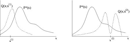
Initialization: Choose an arbitrary point $x_{0}$ to be the first sample, and choose an arbitrary probability density $g(x|y)$ (sometimes written $Q(x|y)$ ) that suggests a candidate for the next sample value $x$ , given the previous sample value $y$ . For the Metropolis algorithm, $g$ must be symmetric; in other words, it must satisfy $g(x|y)=g(y|x)$ . A usual choice is to let $g(x|y)$ be a Gaussian distribution centered at $y$ , so that points closer to $y$ are more likely to be visited next—making the sequence of samples into a random walk. The function $g$ is referred to as the proposal density or jumping distribution.
For each iteration t:
- Generate : Generate a candidate $x'$ for the next sample by picking from the distribution $g(x'|x_{t})$ .
- Calculate : Calculate the acceptance ratio ${\textstyle \alpha =f(x')/f(x_{t})}$ , which will be used to decide whether to accept or reject the candidate. Because f is proportional to the density of P, we have that $\alpha =f(x')/f(x_{t})=P(x')/P(x_{t})$ .
- Accept or Reject :
  - Generate a uniform random number u on [0,1].
  - If $u\leq \alpha$ accept the candidate by setting $x_{t+1}=x'$ ,
  - If $u>\alpha$ reject the candidate and set $x_{t+1}=x_{t}$ , instead.

This algorithm proceeds by randomly attempting to move about the sample space, sometimes accepting the moves and sometimes remaining in place. Note that the acceptance ratio $\alpha$ indicates how probable the new proposed sample is with respect to the current sample, according to the distribution $\displaystyle P(x)$ . If we attempt to move to a point that is more probable than the existing point (i.e. a point in a higher-density region of $\displaystyle P(x)$ ), we will always accept the move. However, if we attempt to move to a less probable point, we will sometimes reject the move, and the more the relative drop in probability, the more likely we are to reject the new point. Thus, we will tend to stay in (and return large numbers of samples from) high-density regions of $\displaystyle P(x)$ , while only occasionally visiting low-density regions. Intuitively, this is why this algorithm works, and returns samples that follow the desired distribution $\displaystyle P(x)$ .

Compared with an algorithm like adaptive rejection sampling^[3] that directly generates independent samples from a distribution, Metropolis–Hastings and other MCMC algorithms have a number of disadvantages:

The samples are correlated. Even though over the long term they do correctly follow $\displaystyle P(x)$ , a set of nearby samples will be correlated with each other and not correctly reflect the distribution. This means that if we want a set of independent samples, we have to throw away the majority of samples and only take every nth sample, for some value of n (typically determined by examining the autocorrelation between adjacent samples). Autocorrelation can be reduced by increasing the jumping width (the average size of a jump, which is related to the variance of the jumping distribution), but this will also increase the likelihood of rejection of the proposed jump. Too large or too small a jumping size will lead to a slow-mixing Markov chain, i.e. a highly correlated set of samples, so that a very large number of samples will be needed to get a reasonable estimate of any desired property of the distribution.
Although the Markov chain eventually converges to the desired distribution, the initial samples may follow a very different distribution, especially if the starting point is in a region of low density. As a result, a burn-in period is typically necessary, where an initial number of samples (e.g. the first 1,000 or so) are thrown away.

On the other hand, most simple rejection sampling methods suffer from the "curse of dimensionality", where the probability of rejection increases exponentially as a function of the number of dimensions. Metropolis–Hastings, along with other MCMC methods, do not have this problem to such a degree, and thus are often the only solutions available when the number of dimensions of the distribution to be sampled is high. As a result, MCMC methods are often the methods of choice for producing samples from hierarchical Bayesian models and other high-dimensional statistical models used nowadays in many disciplines.

In multivariate distributions, the classic Metropolis–Hastings algorithm as described above involves choosing a new multi-dimensional sample point. When the number of dimensions is high, finding the right jumping distribution to use can be difficult, as the different individual dimensions behave in very different ways, and the jumping width (see above) must be "just right" for all dimensions at once to avoid excessively slow mixing. An alternative approach that often works better in such situations, known as Gibbs sampling, involves choosing a new sample for each dimension separately from the others, rather than choosing a sample for all dimensions at once. This is especially applicable when the multivariate distribution is composed out of a set of individual random variables in which each variable is conditioned on only a small number of other variables, as is the case in most typical hierarchical models. The individual variables are then sampled one at a time, with each variable conditioned on the most recent values of all the others. Various algorithms can be used to choose these individual samples, depending on the exact form of the multivariate distribution: some possibilities are the adaptive rejection sampling methods,^[3]^[4]^[5]^[6] the adaptive rejection Metropolis sampling algorithm^[7] or its improvements^[8]^[9] (see matlab code), a simple one-dimensional Metropolis–Hastings step, or slice sampling.

Formal derivation

The purpose of the Metropolis–Hastings algorithm is to generate a collection of states according to a desired distribution $P(x)$ . To accomplish this, the algorithm uses a Markov process which asymptotically reaches a unique stationary distribution $\pi (x)$ such that $\pi (x)=P(x)$ .^[10]

A Markov process is uniquely defined by its transition probabilities, $P(x'|x)$ , the probability of transitioning from any given state, $x$ , to any other given state, $x'$ . It has a unique stationary distribution $\pi (x)$ when the following two conditions are met:^[10]

existence of stationary distribution: there must exist a stationary distribution $\pi (x)$ . A sufficient but not necessary condition is detailed balance which requires that each transition $x\rightarrow x'$ is reversible: for every pair of states $x,x'$ , the probability of being in state x and transitioning to state x' must be equal to the probability of being in state $x'$ and transitioning to state $x$ , $\pi (x)P(x'|x)=\pi (x')P(x|x')$ .
uniqueness of stationary distribution: the stationary distribution $\pi (x)$ must be unique. This is guaranteed by ergodicity of the Markov process, which requires that every state must (1) be aperiodic—the system does not return to the same state at fixed intervals; and (2) be positive recurrent—the expected number of steps for returning to the same state is finite.

The Metropolis–Hastings algorithm involves designing a Markov process (by constructing transition probabilities) which fulfills the two above conditions, such that its stationary distribution $\pi (x)$ is chosen to be $P(x)$ . The derivation of the algorithm starts with the condition of detailed balance:

$P(x'|x)P(x)=P(x',x)=P(x|x')P(x')$

which is re-written as

${\frac {P(x'|x)}{P(x|x')}}={\frac {P(x')}{P(x)}}$ .

The approach is to separate the transition in two sub-steps; the proposal and the acceptance-rejection. The proposal distribution $\displaystyle g(x'|x)$ is the conditional probability of proposing a state $x'$ given $x$ , and the acceptance ratio $\displaystyle A(x',x)$ the probability to accept the proposed state $x'$ . The transition probability can be written as the product of them:

$P(x'|x)=g(x'|x)A(x',x)$ .

Inserting this relation in the previous equation, we have

${\frac {A(x',x)}{A(x,x')}}={\frac {P(x')}{P(x)}}{\frac {g(x|x')}{g(x'|x)}}$ .

The next step in the derivation is to choose an acceptance that fulfils the condition above. One common choice is the Metropolis choice:

$A(x',x)=\min \left(1,{\frac {P(x')}{P(x)}}{\frac {g(x|x')}{g(x'|x)}}\right)$

i.e., we always accept when the acceptance is bigger than 1, and we reject accordingly when the acceptance is smaller than 1. This is the required quantity for the algorithm.

The Metropolis–Hastings algorithm thus consists in the following:

Initialise
1. Pick an initial state $x_{0}$ ;
2. Set $t=0$ ;
Iterate
1. Generate: randomly generate a candidate state x' according to $g(x'|x_{t})$ ;
2. Calculate: calculate the acceptance probability ${\textstyle A(x',x_{t})=\min \left(1,{\frac {P(x')}{P(x_{t})}}{\frac {g(x_{t}|x')}{g(x'|x_{t})}}\right)}$ ;
3. Accept or Reject:
  1. generate a uniform random number $u\in [0,1]$ ;
  2. if $u\leq A(x',x_{t})$ , accept the new state and set $x_{t+1}=x'$ ;
  3. if $u>A(x',x_{t})$ , reject the new state, and copy the old state forward $x_{t+1}=x_{t}$ ;
4. Increment: set ${\textstyle t=t+1}$ ;

Provided that specified conditions are met, the empirical distribution of saved states $x_{0},\ldots ,x_{T}$ will approach $P(x)$ . The number of iterations ( $T$ ) required to effectively estimate $P(x)$ depends on the number of factors, including the relationship between $P(x)$ and the proposal distribution and the desired accuracy of estimation.^[11] For distribution on discrete state spaces, it has to be of the order of the autocorrelation time of the Markov process.^[12]

It is important to notice that it is not clear, in a general problem, which distribution $\displaystyle g(x'|x)$ one should use or the number of iterations necessary for proper estimation; both are free parameters of the method which must be adjusted to the particular problem in hand.

Use in numerical integration

A common use of Metropolis–Hastings algorithm is to compute an integral. Specifically, consider a space $\Omega \subset \mathbb {R}$ and a probability distribution P(x) over $\Omega$ , $x \in \Omega$ . Metropolis-Hastings can estimate an integral of the form of

P(E)=\int _{\Omega }A(x)P(x)dx

where A(x) is an arbitrary function of interest. For example, consider a statistic E(x) and its probability distribution P(E), which is a marginal distribution. Suppose that the goal is to estimate P(E) for E on the tail of P(E). Formally, P(E) can be written as

P(E)=\int _{\Omega }P(E|x)P(x)dx=\int _{\Omega }\delta (E-E(x))P(x)dx=E_{X}(P(E|X))

and, thus, estimating P(E) can be accomplished by estimating the expected value of the indicator function $A_{E}(x)\equiv \mathbf {1} _{E}(x)$ , which is 1 when $E(x)\in [E,E+\Delta E]$ and zero otherwise. Because E is on the tail of P(E), the probability to draw a state x with E(x) on the tail of P(E) is proportional to P(E), which is small by definition. Metropolis-Hastings can be used here to sample (rare) states more likely and thus increase the number of samples used to estimate P(E) on the tails. This can be done e.g. by using a sampling distribution $\pi (x)$ to favor those states (e.g. $\pi (x)\propto e^{aE}$ with a>0).

Step-by-step instructions

Suppose the most recent value sampled is $x_{t}\,$ . To follow the Metropolis–Hastings algorithm, we next draw a new proposal state $x'\,$ with probability density $g(x'|x_{t})\,$ , and calculate a value

a=a_{1}a_{2}\,

where

a_{1}={\frac {P(x')}{P(x_{t})}}\,\!

is the probability (e.g., Bayesian posterior) ratio between the proposed sample $x'\,$ and the previous sample $x_{t}\,$ , and

a_{2}={\frac {g(x_{t}|x')}{g(x'|x_{t})}}

is the ratio of the proposal density in two directions (from $x_{t}\,$ to $x'\,$ and vice versa). This is equal to 1 if the proposal density is symmetric. Then the new state $\displaystyle x_{t+1}$ is chosen according to the following rules.

{\begin{matrix}{\mbox{If }}a\geq 1:&\\&x_{t+1}=x',\end{matrix}}

{\begin{matrix}{\mbox{else}}&\\&x_{t+1}=\left\{{\begin{array}{lr}x'&{\mbox{ with probability }}a\\x_{t}&{\mbox{ with probability }}1-a.\end{array}}\right.\end{matrix}}

The Markov chain is started from an arbitrary initial value $\displaystyle x_{0}$ and the algorithm is run for many iterations until this initial state is "forgotten". These samples, which are discarded, are known as burn-in. The remaining set of accepted values of $x$ represent a sample from the distribution $P(x)$ .

The algorithm works best if the proposal density matches the shape of the target distribution $\displaystyle P(x)$ from which direct sampling is difficult, that is $g(x'|x_{t})\approx P(x')\,\!$ . If a Gaussian proposal density $\displaystyle g$ is used the variance parameter $\displaystyle \sigma ^{2}$ has to be tuned during the burn-in period. This is usually done by calculating the acceptance rate, which is the fraction of proposed samples that is accepted in a window of the last $\displaystyle N$ samples. The desired acceptance rate depends on the target distribution, however it has been shown theoretically that the ideal acceptance rate for a one-dimensional Gaussian distribution is approx 50%, decreasing to approx 23% for an $\displaystyle N$ -dimensional Gaussian target distribution.^[13]

If $\displaystyle \sigma ^{2}$ is too small the chain will mix slowly (i.e., the acceptance rate will be high but successive samples will move around the space slowly and the chain will converge only slowly to $\displaystyle P(x)$ ). On the other hand, if $\displaystyle \sigma ^{2}$ is too large the acceptance rate will be very low because the proposals are likely to land in regions of much lower probability density, so $\displaystyle a_{1}$ will be very small and again the chain will converge very slowly.

The result of three Markov chains running on the 3D Rosenbrock function using the Metropolis-Hastings algorithm. The algorithm samples from regions where the posterior probability is high and the chains begin to mix in these regions. The approximate position of the maximum has been illuminated. Note that the red points are the ones that remain after the burn-in process. The earlier ones have been discarded.

References

↑ Hastings, W.K. (1970). "Monte Carlo Sampling Methods Using Markov Chains and Their Applications". Biometrika. 57 (1): 97&ndash, 109. Bibcode:1970Bimka..57...97H. doi:10.1093/biomet/57.1.97. JSTOR 2334940. Zbl 0219.65008.
↑ Teller, Edward. Memoirs: A Twentieth-Century Journey in Science and Politics. Perseus Publishing, 2001, p. 328
1 2 Gilks, W. R.; Wild, P. (1992-01-01). "Adaptive Rejection Sampling for Gibbs Sampling". Journal of the Royal Statistical Society. Series C (Applied Statistics). 41 (2): 337–348. doi:10.2307/2347565. JSTOR 2347565.
↑ Görür, Dilan; Teh, Yee Whye (2011-01-01). "Concave-Convex Adaptive Rejection Sampling". Journal of Computational and Graphical Statistics. 20 (3): 670–691. doi:10.1198/jcgs.2011.09058. ISSN 1061-8600.
↑ Hörmann, Wolfgang (1995-06-01). "A Rejection Technique for Sampling from T-concave Distributions". ACM Trans. Math. Softw. 21 (2): 182–193. doi:10.1145/203082.203089. ISSN 0098-3500.
↑ Martino, Luca; Míguez, Joaquín (2010-08-25). "A generalization of the adaptive rejection sampling algorithm". Statistics and Computing. 21 (4): 633–647. doi:10.1007/s11222-010-9197-9. ISSN 0960-3174.
↑ Gilks, W. R.; Best, N. G.; Tan, K. K. C. (1995-01-01). "Adaptive Rejection Metropolis Sampling within Gibbs Sampling". Journal of the Royal Statistical Society. Series C (Applied Statistics). 44 (4): 455–472. doi:10.2307/2986138. JSTOR 2986138.
↑ Martino, L.; Read, J.; Luengo, D. (2015-06-01). "Independent Doubly Adaptive Rejection Metropolis Sampling Within Gibbs Sampling". IEEE Transactions on Signal Processing. 63 (12): 3123–3138. arXiv:1205.5494. Bibcode:2015ITSP...63.3123M. doi:10.1109/TSP.2015.2420537. ISSN 1053-587X.
↑ Meyer, Renate; Cai, Bo; Perron, François (2008-03-15). "Adaptive rejection Metropolis sampling using Lagrange interpolation polynomials of degree 2". Computational Statistics & Data Analysis. 52 (7): 3408–3423. doi:10.1016/j.csda.2008.01.005.
1 2 Robert, Christian; Casella, George (2004). Monte Carlo Statistical Methods. Springer. ISBN 0387212396.
↑ Raftery, Adrian E., and Steven Lewis. "How Many Iterations in the Gibbs Sampler?." In Bayesian Statistics 4. 1992.
↑ Newman, M. E. J.; Barkema, G. T. (1999). Monte Carlo Methods in Statistical Physics. USA: Oxford University Press. ISBN 0198517971.
↑ Roberts, G.O.; Gelman, A.; Gilks, W.R. (1997). "Weak convergence and optimal scaling of random walk Metropolis algorithms". Ann. Appl. Probab. 7 (1): 110&ndash, 120. CiteSeerX 10.1.1.717.2582. doi:10.1214/aoap/1034625254.
Rosenbluth, Marshall. "Oral History Transcript". American Institute of Physics
J.E. Gubernatis (2005). "Marshall Rosenbluth and the Metropolis Algorithm". Physics of Plasmas. 12 (5): 057303. Bibcode:2005PhPl...12e7303G. doi:10.1063/1.1887186.

External links

Metropolis-Hastings algorithm on xβ
Matlab implementation of Random-Walk Metropolis
R implementation of Random-Walk Metropolis
IA2RMS is a Matlab code of the Independent Doubly Adaptive Rejection Metropolis Sampling method for drawing from the full-conditional densities within a Gibbs sampler.

This article is issued from Wikipedia. The text is licensed under Creative Commons - Attribution - Sharealike. Additional terms may apply for the media files.

[Hastings-1] Hastings, W.K. (1970). "Monte Carlo Sampling Methods Using Markov Chains and Their Applications". Biometrika. 57 (1): 97&ndash, 109. Bibcode:1970Bimka..57...97H. doi:10.1093/biomet/57.1.97. JSTOR 2334940. Zbl 0219.65008.

[Teller-2] Teller, Edward. Memoirs: A Twentieth-Century Journey in Science and Politics. Perseus Publishing, 2001, p. 328

[:0-3] 1 2 Gilks, W. R.; Wild, P. (1992-01-01). "Adaptive Rejection Sampling for Gibbs Sampling". Journal of the Royal Statistical Society. Series C (Applied Statistics). 41 (2): 337–348. doi:10.2307/2347565. JSTOR 2347565.

[4] Görür, Dilan; Teh, Yee Whye (2011-01-01). "Concave-Convex Adaptive Rejection Sampling". Journal of Computational and Graphical Statistics. 20 (3): 670–691. doi:10.1198/jcgs.2011.09058. ISSN 1061-8600.

[5] Hörmann, Wolfgang (1995-06-01). "A Rejection Technique for Sampling from T-concave Distributions". ACM Trans. Math. Softw. 21 (2): 182–193. doi:10.1145/203082.203089. ISSN 0098-3500.

[6] Martino, Luca; Míguez, Joaquín (2010-08-25). "A generalization of the adaptive rejection sampling algorithm". Statistics and Computing. 21 (4): 633–647. doi:10.1007/s11222-010-9197-9. ISSN 0960-3174.

[7] Gilks, W. R.; Best, N. G.; Tan, K. K. C. (1995-01-01). "Adaptive Rejection Metropolis Sampling within Gibbs Sampling". Journal of the Royal Statistical Society. Series C (Applied Statistics). 44 (4): 455–472. doi:10.2307/2986138. JSTOR 2986138.

[8] Martino, L.; Read, J.; Luengo, D. (2015-06-01). "Independent Doubly Adaptive Rejection Metropolis Sampling Within Gibbs Sampling". IEEE Transactions on Signal Processing. 63 (12): 3123–3138. arXiv:1205.5494. Bibcode:2015ITSP...63.3123M. doi:10.1109/TSP.2015.2420537. ISSN 1053-587X.

[9] Meyer, Renate; Cai, Bo; Perron, François (2008-03-15). "Adaptive rejection Metropolis sampling using Lagrange interpolation polynomials of degree 2". Computational Statistics & Data Analysis. 52 (7): 3408–3423. doi:10.1016/j.csda.2008.01.005.

[Roberts_Casella-10] 1 2 Robert, Christian; Casella, George (2004). Monte Carlo Statistical Methods. Springer. ISBN 0387212396.

[11] Raftery, Adrian E., and Steven Lewis. "How Many Iterations in the Gibbs Sampler?." In Bayesian Statistics 4. 1992.

[Newman_Barkema-12] Newman, M. E. J.; Barkema, G. T. (1999). Monte Carlo Methods in Statistical Physics. USA: Oxford University Press. ISBN 0198517971.

[Roberts-13] Roberts, G.O.; Gelman, A.; Gilks, W.R. (1997). "Weak convergence and optimal scaling of random walk Metropolis algorithms". Ann. Appl. Probab. 7 (1): 110&ndash, 120. CiteSeerX 10.1.1.717.2582. doi:10.1214/aoap/1034625254.

[Rosenbluth-14] Rosenbluth, Marshall. "Oral History Transcript". American Institute of Physics

[Gubernatis-15] J.E. Gubernatis (2005). "Marshall Rosenbluth and the Metropolis Algorithm". Physics of Plasmas. 12 (5): 057303. Bibcode:2005PhPl...12e7303G. doi:10.1063/1.1887186.