Fraunhofer diffraction equation
In optics, the Fraunhofer diffraction equation is used to model the diffraction of waves when the diffraction pattern is viewed at a long distance from the diffracting object, and also when it is viewed at the focal plane of an imaging lens.[1][2]
The equation was named in honour of Joseph von Fraunhofer although he was not actually involved in the development of the theory.[3]
This article gives the equation in various mathematical forms, and provides detailed calculations of the Fraunhofer diffraction pattern for several different forms of diffracting apertures, specially for normally incident monochromatic plane wave. A qualitative discussion of Fraunhofer diffraction can be found elsewhere.
Definition
When a beam of light is partly blocked by an obstacle, some of the light is scattered around the object, and light and dark bands are often seen at the edge of the shadow – this effect is known as diffraction.[4] The Kirchhoff diffraction equation provides an expression, derived from the wave equation, which describes the wave diffracted by an aperture; analytical solutions to this equation are not available for most configurations.[5]
The Fraunhofer diffraction equation is an approximation which can be applied when the diffracted wave is observed in the far field, and also when a lens is used to focus the diffracted light; in many instances, a simple analytical solution is available to the Fraunhofer equation – several of these are derived below.
In Cartesian co-ordinates

If the aperture is in x'y' plane, with the origin in the aperture and is illuminated by a monochromatic wave, of wavelength λ, wavenumber k with complex amplitude A(x ',y '), and the diffracted wave is observed in the x,y,z plane where l,m are the direction cosines of the point x,y with respect to the origin, the complex amplitude U(x,y) of the diffracted wave is given by the Fraunhofer diffraction equation as:[6]


It can be seen from this equation that the form of the diffraction pattern depends only on the direction of viewing, so the diffraction pattern changes in size but not in form with change of viewing distance.
The Fraunhofer diffraction equation can be expressed in a variety of mathematically equivalent forms. For example:[7]


It can be seen that the integral in the above equations is the Fourier transform of the aperture function evaluated at frequencies[8]


Thus, we can also write the equation in terms of a Fourier transform as:
![U(x,y,z)\propto {\hat f}[A(x',y')]_{{f_{x}f_{y}}}](../I/m/827da252077afa33af507a455469cc5a49e918ea.svg)
where  is the Fourier transform of A. The Fourier transform formulation can be very useful in solving diffraction problems.
Another form is:

where r and r' represent the observation point and a point in the aperture respectively, k0 and k represent the wave vectors of the disturbance at the aperture and of the diffracted waves respectively, and a0(r' ) represents the magnitude of the disturbance at the aperture.
In polar co-ordinates
When the diffracting aperture has circular symmetry, it is useful to use polar rather than Cartesian co-ordinates.[9]
A point in the aperture has co-ordinates ρ,ω giving:

and

The complex amplitude at ρ' is given by A(ρ), and the area dx dy converts to ρ′ dρ′ dω′, giving

Using the integral representation of the Bessel function:[10]

we have

where the integration over ω gives 2π since the equation is circularly symmetric, i.e. there is no dependence on ω.
In this case, we have U(ρ,z) equal to the Fourier–Bessel or Hankel transform of the aperture function, A(ρ)
Example
Here are given examples of Fraunhofer diffraction with a normally incident monochromatic plane wave.
In each case, the diffracting object is located in the z = 0 plane, and the complex amplitude of the incident plane wave is given by

where
- a is the magnitude of the wave disturbance,
- λ is the wavelength,
- c is the velocity of light,
- t is the time
- k = 2 π/λ is the wave number
and the phase is zero at time t = 0.
The time dependent factor is omitted throughout the calculations, as it remains constant, and is averaged out when the intensity is calculated. The intensity at r is proportional to the amplitude times its complex conjugate

These derivations can be found in most standard optics books, in slightly different forms using varying notations. A reference is given for each of the systems modelled here. The Fourier transforms used can be found here.
Slit of infinite depth
.svg.png)
The aperture is a slit of width W which is located along the y-axis,
- Solution by integration
Assuming the centre of the slit is located at x = 0, the first equation above, for all values of y, is:[11]
![{\displaystyle {\begin{aligned}U(x,z)&=a\int _{-W/2}^{W/2}e^{{-2\pi ixx'}/(\lambda z)}\,dx'\\[4pt]&=-{\frac {a\lambda z}{2\pi ix}}\left|e^{{-2\pi ixx'}/(\lambda z)}\right|_{-W/2}^{W/2}\end{aligned}}}](../I/m/e72384a0879ebabd96de73062a27e81e06a33820.svg)
Using Euler's formula, this can be simplified to:
![{\displaystyle {\begin{aligned}U(x,z)&=aW{\frac {\sin \left[{\frac {\pi Wx}{\lambda z}}\right]}{\frac {\pi Wx}{\lambda z}}}\\&=aW\operatorname {sinc} {\frac {\pi Wx}{\lambda z}}\end{aligned}}}](../I/m/9e8079719e70e2006ec4eee168c47fcc08c8c128.svg)
where sinc(p) = sin(p)/p. It should be noted that the sinc function is sometimes defined as sin(πp)/πp and this may cause confusion when looking at derivations in different texts.
This can also be written as:
![{\displaystyle U(\theta )=aW\operatorname {sinc} \left[{\frac {\pi W\sin \theta }{\lambda }}\right]}](../I/m/559aa3cd80b0bd5e374a5123fbc761f1842a9809.svg)
where θ is the angle between z-axis and the line joining x to the origin and sin θ ≈ x/z when θ << 1.
- Fourier transform solution
The slit can be represented by the rect function as:[12]

The Fourier transform of this function is given by

where ξ is the Fourier transform frequency, and the sinc function is here defined as sin(πx)/(πx)
The Fourier transform frequency here is x/λz, giving

Note that the sinc function is here defined as sin(x)/(x) to maintain consistency.
- Intensity
The intensity is proportional to the square of the amplitude, and is then[13]
![{\displaystyle {\begin{aligned}I(\theta )&\propto \operatorname {sinc} ^{2}\left[{\frac {\pi W\sin \theta }{\lambda }}\right]\\&\propto \operatorname {sinc} ^{2}\left[{\frac {kW\sin \theta }{2}}\right]\end{aligned}}}](../I/m/23f8940e510be8fb31eae497643108e665466da3.svg)
Apertures
Rectangular aperture
When a slit of width W and height H is illuminated normally by a monochromatic plane wave of wavelength λ, the complex amplitude can be found using similar analyses to those in the previous section, applied over two independent dimensions as:[14][15]

The intensity is given by

where θ and φ are the angles between the x and z axes and the y and z axes, respectively.
In practice, all slits are of finite length and will therefore produce diffraction on both directions. If the length of the slit is much greater than its width, then the spacing of the horizontal diffraction fringes will be much less than the spacing of the vertical fringes. If the illuminating beam does not illuminate the whole length of the slit, the spacing of the horizontal fringes is determined by the dimensions of the laser beam. Close examination of the two-slit pattern below shows that there are very fine horizontal diffraction fringes above and below the main spot, as well as the more obvious vertical fringes.
Circular aperture
The aperture has diameter W. The complex amplitude in the observation plane is given by

- Solution by integration
Using the recurrence relationship[16]
![{\frac {d}{dx}}\left[x^{{n+1}}J_{{n+1}}(x)\right]=x^{{n+1}}J_{n}(x)](../I/m/53af98c5968e3a20a51824a97facabd99cf02546.svg)
to give

If we substitute

and the limits of the integration become 0 and πρW/λz, we get

Putting ρ/z = sin θ, we get

- Solution using Fourier–Bessel transform
We can write the aperture function as a step function

The Fourier–Bessel transform for this function is given by the relationship
![~F[\Pi (r/a)]={\frac {2\pi J_{1}(qa)}{q}}](../I/m/7db3e5fda430b68180a73c61d3b4e2873ea2f21b.svg)
where q/2π is the transform frequency which is equal to ρ/λz and a = W/2.
Thus, we get

- Intensity
The intensity is given by:[17]
![{\begin{aligned}I(\theta )&\propto \left[{\frac {J_{1}(\pi W\sin \theta /\lambda )}{\pi W\sin \theta /\lambda )}}\right]^{2}\\&\propto \left[{\frac {J_{1}(kW\sin \theta /2)}{(kW\sin \theta /2)}}\right]^{2}\end{aligned}}](../I/m/b3ceaff3087d33326acc12336bcbb55937f59dd2.svg)
Form of the diffraction pattern
This known as the Airy diffraction pattern
The diffracted pattern is symmetric about the normal axis.
Aperture with a Gaussian profile

An aperture with a Gaussian profile, for example, a photographic slide whose transmission has a Gaussian variation, so that the amplitude at a point in the aperture located at a distance r' from the origin is given by
![A(\rho ')=\exp {\left(-\left[{\frac {\rho '}{\sigma }}\right]^{2}\right)}](../I/m/7f9227f546a228a2422dc0d79931e00110a6571a.svg)
giving
![U(\rho ,z)=2\pi a\int _{0}^{\infty }\exp {\left(-\left[{\frac {\rho '}{\sigma }}\right]^{2}\right)}J_{0}(2\pi \rho '\rho /\lambda z)\rho '\,d\rho '](../I/m/706846318f25ca95b0bc6e846848f65526fff1dd.svg)
- Solution using Fourier–Bessel transform
The Fourier–Bessel or Hankel transform is defined as

where Jν is the Bessel function of the first kind of order ν with ν ≥ −1/2.
The Hankel transform is
![F_{\nu }[e^{{(ar)^{2}/2}}]={\frac {e^{{-k^{2}/2a^{2}}}}{a^{2}}}](../I/m/5ee69c2db51bfe8c70c8bed777ce3e7a8763a82d.svg)
giving
![{\begin{aligned}U(\rho ,z)&\propto e^{{-[{\frac {\pi \rho \sigma }{\lambda z}}]^{2}}}\end{aligned}}](../I/m/4b85ac63a6a27e862967e10cdfac9d9394cc1d4e.svg)
and
![U(\theta )\propto e^{{-[{\frac {\pi \sigma \sin \theta }{\lambda }}]^{2}}}](../I/m/9daaa66eb3194fa96d0d2b45924de33305597b9b.svg)
- Intensity
The intensity is given by:[18]
![I(\theta )\propto e^{{-[{\frac {2\pi \sigma \sin \theta }{\lambda }}]}}](../I/m/4b71303d412e20aa206d4aa5d245c7663d357a6c.svg)
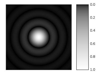
This function is plotted on the right, and it can be seen that, unlike the diffraction patterns produced by rectangular or circular apertures, it has no secondary rings. This can be used in a process called apodization - the aperture is covered by a filter whose transmission varies as a Gaussian function, giving a diffraction pattern with no secondary rings.:[19][20]
Slits
Two slits
The pattern which occurs when light diffracted from two slits overlaps is of considerable interest in physics, firstly for its importance in establishing the wave theory of light through Young's interference experiment, and secondly because of its role as a thought experiment in double-slit experiment in quantum mechanics.
Narrow slits
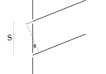

Assume we have two long slits illuminated by a plane wave of wavelength λ. The slits are in the z = 0 plane, parallel to the y axis, separated by a distance S and are symmetrical about the origin. The width of the slits is small compared with the wavelength.
- Solution by integration
The incident light is diffracted by the slits into uniform spherical waves. The waves travelling in a given direction θ from the two slits have differing phases. The phase of the waves from the upper and lower slits relative to the origin is given by (2π/λ)(S/2)sin θ and -(2π/λ)(S/2)sin θ
The complex amplitude of the summed waves is given by:[21]

- Solution using Fourier transform
The aperture can be represented by the function:[22]
![~a[\delta {(x-S/2)}+\delta {(x+S/2)}]](../I/m/0ec04a282225aefd5b61baa6adbf32420b014d10.svg)
where δ is the delta function.
We have
![{\hat {f}}[\delta (x)]=1](../I/m/d765dbe290d97d5ba5bf4e5056efe055dbfb1085.svg)
and
![{\hat {f}}[g(x-a)]=e^{{-2\pi iaf_{x}}}{\hat {f}}[g(x)]](../I/m/d149808065d9b4830b9cf4159b645df22c7b1938.svg)
giving
![{\displaystyle {\begin{aligned}U(x,z)&={\hat {f}}[\delta {(x-S/2)}+\delta {(x+S/2)}]\\&=e^{-i\pi Sx/2\lambda }+e^{i\pi Sx/2\lambda }\\&=2\cos {\frac {\pi Sx}{2\lambda }}\end{aligned}}}](../I/m/f1b84838573ac106cc9dd18094ccaff7fd4f95ab.svg)

This is the same expression as that derived above by integration.
- Intensity
This gives the intensity of the combined waves as:[23]
![{\displaystyle {\begin{aligned}I(\theta )&\propto \cos ^{2}\left[{\frac {\pi S\sin \theta }{\lambda }}\right]\\&\propto \cos ^{2}{\left[{\frac {kS\sin \theta }{2}}\right]}\end{aligned}}}](../I/m/0555e66edb580919787e84589ccad857b4a20298.svg)
Slits of finite width
The width of the slits, W is finite.
- Solution by integration
The diffracted pattern is given by:[24]
![{\displaystyle {\begin{aligned}U(\theta )&=a\left[e^{\frac {i\pi S\sin \theta }{\lambda }}+e^{-{\frac {i\pi S\sin \theta }{\lambda }}}\right]\int _{-W/2}^{W/2}e^{{-2\pi ix'\sin \theta }/(\lambda )}\,dx'\\&=2a\cos {\frac {\pi S\sin \theta }{\lambda }}W\operatorname {sinc} {\frac {\pi W\sin \theta }{\lambda }}\end{aligned}}}](../I/m/c89b11bc6e39f37e085bdcd06c0f67b05bc6558d.svg)
- Solution using Fourier transform
The aperture function is given by:[25]
![{\displaystyle a\left[\operatorname {rect} \left({\frac {x-S/2}{W}}\right)+\operatorname {rect} \left({\frac {x+S/2}{W}}\right)\right]}](../I/m/ec0420b6d06178713fce93b12429ac4197a2f48f.svg)
The Fourier transform of this function is given by
where ξ is the Fourier transform frequency, and the sinc function is here defined as sin(πx)/(πx)
and
We have
![{\displaystyle {\begin{aligned}U(x,z)&={\hat {f}}\left[a\left[\operatorname {rect} \left({\frac {x-S/2}{W}}\right)+\operatorname {rect} \left({\frac {x+S/2}{W}}\right)\right]\right]\\&=2W\left[e^{-i\pi Sx/\lambda z}+e^{i\pi Sx/\lambda z}\right]{\frac {\sin {\frac {\pi Wx}{\lambda z}}}{\frac {\pi Wx}{\lambda z}}}\\&=2a\cos {\frac {\pi Sx}{\lambda z}}W\operatorname {sinc} {\frac {\pi Wx}{\lambda z}}\end{aligned}}}](../I/m/ed93beb3da56f961ac6deee763d1df3d6d01833a.svg)
or

This is the same expression as was derived by integration.
- Intensity
The intensity is given by:[26]
![{\displaystyle {\begin{aligned}I(\theta )&\propto \cos ^{2}\left[{\frac {\pi S\sin \theta }{\lambda }}\right]\operatorname {sinc} ^{2}\left[{\frac {\pi W\sin \theta }{\lambda }}\right]\\&\propto \cos ^{2}\left[{\frac {kS\sin \theta }{2}}\right]\operatorname {sinc} ^{2}\left[{\frac {kW\sin \theta }{2}}\right]\end{aligned}}}](../I/m/197ee093ddcc5286e0308f731d07125134c2c918.svg)
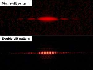
It can be seen that the form of the intensity pattern is the product of the individual slit diffraction pattern, and the interference pattern which would be obtained with slits of negligible width. This is illustrated in the image at the right which shows single slit diffraction by a laser beam, and also the diffraction/interference pattern given by two identical slits.
Gratings
A grating is defined in Born and Wolf as "any arrangement which imposes on an incident wave a periodic variation of amplitude or phase, or both".[27]
Narrow slit grating
A simple grating consists of a screen with N slits whose width is significantly less than the wavelength of the incident light with slit separation of S.
- Solution by integration
The complex amplitude of the diffracted wave at an angle θ is given by:[28]

since this is the sum of a geometric series.
- Solution using Fourier transform
The aperture is given by

The Fourier transform of this function is:[29]
![{\begin{aligned}{\hat {f}}\left[\sum _{{n=0}}^{{N}}\delta (x-nS)\right]&=\sum _{{n=0}}^{{N}}e^{{-if_{x}nS}}\\&={\frac {1-e^{{-i2\pi NS\sin \theta /\lambda }}}{1-e^{{-i2\pi S\sin \theta /\lambda }}}}\end{aligned}}](../I/m/bb7e43ac1a73b794dd839934e03fcf0f92c6635d.svg)
- Intensity
The intensity is given by:[30]

This function has a series of maxima and minima. There are regularly spaced "principal maxima", and a number of much smaller maxima in between the principal maxima. The principal maxima occur when

and the main diffracted beams therefore occur at angles:

This is the grating equation for normally incident light.
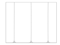
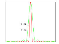
The number of small intermediate maxima is equal to the number of slits, N − 1 and their size and shape is also determined by N.
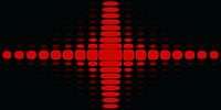
The form of the pattern for N=50 is shown in the first figure .
The detailed structure for 20 and 50 slits gratings are illustrated in the second diagram.
Finite width slit grating
The grating now has N slits of width W and spacing S
- Solution using integration
The amplitude is given by:[31]

- Solution using Fourier transform
The aperture function can be written as:[32]
![{\displaystyle \sum _{n=1}^{N}\operatorname {rect} \left[{\frac {x'-nS}{W}}\right]}](../I/m/5ae41623b808fac1fef16c4811779c8e529cde5d.svg)
Using the convolution theorem, which says that if we have two functions f(x) and g(x), and we have

where ∗ denotes the convolution operation, then we also have

we can write the aperture function as

The amplitude is then given by the Fourier transform of this expression as:
![{\displaystyle {\begin{aligned}U(x,z)&={\hat {f}}[\operatorname {rect} (x'/W)]{\hat {f}}\left[\sum _{n=0}^{N}\delta (x'-nS)\right]\\&=a\operatorname {sinc} \left({\frac {W\sin \theta }{\lambda }}\right){\frac {1-e^{-i2\pi NS\sin \theta /\lambda }}{1-e^{-i2\pi S\sin \theta /\lambda }}}\end{aligned}}}](../I/m/002f00cd39861a48319b8e2d6d8899e7b113d221.svg)
- Intensity
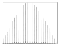
The intensity is given by:[33]

The diagram shows the diffraction pattern for a grating with 20 slits, where the width of the slits is 1/5th of the slit separation. The size of the main diffracted peaks is modulated with the diffraction pattern of the individual slits.
Other gratings
The Fourier transform method above can be used to find the form of the diffraction for any periodic structure where the Fourier transform of the structure is known. Goodman[34] uses this method to derive expressions for the diffraction pattern obtained with sinusoidal amplitude and phase modulation gratings. These are of particular interest in holography.
Extensions
Non-normal illumination
If the aperture is illuminated by a mono-chromatic plane wave incident in a direction (l0,m0, n0), the first version of the Fraunhofer equation above becomes:[35]
![{\displaystyle {\begin{aligned}U(x,y,z)&\propto \iint _{\text{Aperture}}\,A(x',y')e^{-i{\frac {2\pi }{\lambda }}[(l-l_{0})x'+(m-m_{0})y']}\,dx'\,dy'\\&\propto \iint _{\text{Aperture}}\,A(x',y')e^{-ik[(l-l_{0})x'+(m-m_{0})y']}\,dx'\,dy'\end{aligned}}}](../I/m/3bff95fbf72e3482e2e46a78edf8f8cec7e51251.svg)
The equations used to model each of the systems above are altered only by changes in the constants multiplying x and y, so the diffracted light patterns will have the form, except that they will now be centred around the direction of the incident plane wave.
The grating equation becomes[36]

Non-monochromatic illumination
In all of the above examples of Fraunhofer diffraction, the effect of increasing the wavelength of the illuminating light is to reduce the size of the diffraction structure, and conversely, when the wavelength is reduced, the size of the pattern increases. If the light is not mono-chromatic, i.e. it consists of a range of different wavelengths, each wavelength is diffracted into a pattern of a slightly different size to its neighbours. If the spread of wavelengths is significantly smaller than the mean wavelength, the individual patterns will vary very little in size, and so the basic diffraction will still appear with slightly reduced contrast. As the spread of wavelengths is increased, the number of "fringes" which can be observed is reduced.
See also
References
- ↑ Born & Wolf, 1999, p 427.
- ↑ Jenkins & White, 1957, p 288
- ↑ http://scienceworld.wolfram.com/biography/Fraunhofer.html
- ↑ Heavens & Ditchburn, 1996, p 62
- ↑ Born & Wolf, 2002, p 425
- ↑ Lipson et al., 2011, eq(8.8) p 231
- ↑ Hecht, 2002, eq (11.63), p 529
- ↑ Hecht, 2002, eq(11.67), p 540
- ↑ Born & Wolf, 2002, Section 8.5.2, eqs (6–8), p 439
- ↑ Abramowitz & Stegun, 1964, Section 9.1.21, p 360
- ↑ Born & Wolf, 1999, Section 8.5.1 p 436
- ↑ Hecht, 2002, p 540
- ↑ Hecht, 2002, eqs (10.17) (10.18), p 453
- ↑ Longhurst, 1967, p 217
- ↑ Goodman, eq(4.28), p 76
- ↑ Whittaker and Watson, example 2, p 360
- ↑ Hecht, 2002, eq (10.56), p 469
- ↑ Hecht, 2002, eq (11.2), p 521
- ↑ Heavens & Ditchburn, 1991, p 68
- ↑ Hecht, 2002, Figure (11.33), p 543
- ↑ Jenkins & White, 1957, eq (16c), p 312
- ↑ Hecht, 2002, eq (11.4328), p 5
- ↑ Lipson et al., 2011, eq (9.3), p 280
- ↑ Hecht, 2002, Section 10.2.2, p 451
- ↑ Hecht, 2002, p 541
- ↑ Jenkins and White, 1967, eq (16c), p 313
- ↑ Born & Wolf, 1999, Section 8.6.1, p 446
- ↑ Jenkins & White, 1957, eq (17a), p 330
- ↑ Lipson et al., 2011, eq(4.41), p 106
- ↑ Born & Wolf, 1999, eq(5a), p 448
- ↑ Born & Wolf, Section 8.6.1, eq (5), p 448
- ↑ Hecht, The array theorem, p 543
- ↑ Born & Wolf, 2002, Section 8.6, eq (10), p 451
- ↑ Goodman, 2005, Sections 4.4.3 and 4.4.4, p 78
- ↑ Lipson et al., 2011, Section 8.2.2, p 232
- ↑ Born & Wolf, 1999, eq (8), p 449
Reference sources
- Abramowitz Milton & Stegun Irene A,1964, Dover Publications Inc, New York.
- Born M & Wolf E, Principles of Optics, 1999, 7th Edition, Cambridge University Press, ISBN 978-0-521-64222-4
- Goodman Joseph, 2005, Introduction to Fourier Optics, Roberts & Co. ISBN 0-9747077-2-4 or online here
- Heavens OS and Ditchburn W, 1991, Insight into Optics, Longman and Sons, Chichester ISBN 978-0-471-92769-3
- Hecht Eugene, Optics, 2002, Addison Wesley, ISBN 0-321-18878-0
- Jenkins FA & White HE, 1957, Fundamentals of Optics, 3rd Edition, McGraw Hill, New York
- Lipson A, Lipson SG, Lipson H, 2011, Optical Physics, 4th ed., Cambridge University Press, ISBN 978-0-521-49345-1
- Longhurst RS, 1967, Geometrical and Physical Optics, 2nd Edition, Longmans, London
- Whittaker and Watson, 1962, Modern Analysis, Cambridge University Press.