Binary search algorithm
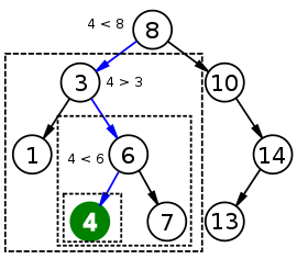
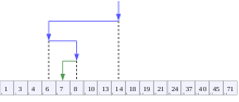 Visualization of the binary search algorithm where 7 is the target value | |
| Class | Search algorithm |
|---|---|
| Data structure | Array |
| Worst-case performance | O(log n) |
| Best-case performance | O(1) |
| Average performance | O(log n) |
| Worst-case space complexity | O(1) |
In computer science, binary search, also known as half-interval search,[1] logarithmic search,[2] or binary chop,[3] is a search algorithm that finds the position of a target value within a sorted array.[4][5] Binary search compares the target value to the middle element of the array. If they are not equal, the half in which the target cannot lie is eliminated and the search continues on the remaining half, again taking the middle element to compare to the target value, and repeating this until the target value is found. If the search ends with the remaining half being empty, the target is not in the array. Even though the idea is simple, implementing binary search correctly requires attention to some subtleties about its exit conditions and midpoint calculation.
Binary search runs in logarithmic time in the worst case, making O(log n) comparisons, where n is the number of elements in the array, the O is Big O notation, and log is the logarithm. Binary search takes constant (O(1)) space, meaning that the space taken by the algorithm is the same for any number of elements in the array.[6] Binary search is faster than linear search except for small arrays, but the array must be sorted first. Although specialized data structures designed for fast searching, such as hash tables, can be searched more efficiently, binary search applies to a wider range of problems.
There are numerous variations of binary search. In particular, fractional cascading speeds up binary searches for the same value in multiple arrays. Fractional cascading efficiently solves a number of search problems in computational geometry and in numerous other fields. Exponential search extends binary search to unbounded lists. The binary search tree and B-tree data structures are based on binary search.
Algorithm
Binary search works on sorted arrays. Binary search begins by comparing the middle element of the array with the target value. If the target value matches the middle element, its position in the array is returned. If the target value is less than the middle element, the search continues in the lower half of the array. If the target value is greater than the middle element, the search continues in the upper half of the array. By doing this, the algorithm eliminates the half in which the target value cannot lie in each iteration.[7]
Procedure
Given an array A of n elements with values or records A0, A1, ..., An−1, sorted such that A0 ≤ A1 ≤ ... ≤ An−1, and target value T, the following subroutine uses binary search to find the index of T in A.[7]
- Set L to 0 and R to n − 1.
- If L > R, the search terminates as unsuccessful.
- Set m (the position of the middle element) to the floor of (L + R) / 2, which is the greatest integer less than or equal to (L + R) / 2.
- If Am < T, set L to m + 1 and go to step 2.
- If Am > T, set R to m − 1 and go to step 2.
- Now Am = T, the search is done; return m.
This iterative procedure keeps track of the search boundaries with the two variables L and R. The procedure may be expressed in pseudocode as follows, where the variable names and types remain the same as above, floor is the floor function, and unsuccessful refers to a specific variable that conveys the failure of the search.[7]
function binary_search(A, n, T):
    L := 0
    R := n − 1
    while L <= R:
        m := floor((L + R) / 2)
        if A[m] < T:
            L := m + 1
        else if A[m] > T:
            R := m - 1
        else:
            return m
    return unsuccessful
Alternative procedure
In the above procedure, the algorithm checks whether the middle element (m) is equal to the target (T) in every iteration. Some implementations leave out this check during each iteration. The algorithm would perform this check only when one element is left (when L = R). This results in a faster comparison loop, as one comparison is eliminated per iteration. However, it requires one more iteration on average.[8]
Hermann Bottenbruch published the first implementation to leave out this check in 1962.[8][9]
- Set L to 0 and R to n − 1.
- If L = R, go to step 6.
- Set m (the position of the middle element) to the ceiling of (L + R) / 2, which is the least integer greater than or equal to (L + R) / 2..
- If Am > T, set R to m − 1 and go to step 2.
- Set L to m and go to step 2.
- Now L = R, the search is done. If AL = T, return L. Otherwise, the search terminates as unsuccessful.
Duplicate elements
The procedure may return any index whose element is equal to the target value, even if there are duplicate elements in the array. For example, if the array to be searched was [1, 2, 3, 4, 4, 5, 6, 7] and the target was 4, then it would be correct for the algorithm to either return the 4th (index 3) or 5th (index 4) element. The regular procedure would return the 4th element (index 3). However, it is sometimes necessary to find the leftmost element or the rightmost element if the target value is duplicated in the array. In the above example, the 4th element is the leftmost element of the value 4, while the 5th element is the rightmost element of the value 4. The alternative procedure above will always return the index of the rightmost element if an element is duplicated in the array.[9]
Procedure for finding the leftmost element
To find the leftmost element, the following procedure can be used:[10]
- Set L to 0 and R to n.
- If L ≥ R, go to step 6.
- Set m (the position of the middle element) to the floor of (L + R) / 2, which is the greatest integer less than or equal to (L + R) / 2
- If Am < T, set L to m + 1 and go to step 2.
- Otherwise, if Am ≥ T, set R to m and go to step 2.
- Now L = R, the search is done, return L.
If L < n and AL = T, then AL is the leftmost element that equals T. Even if T is not in the array, L is the rank of T in the array, or the number of elements in the array that are less than T.
Where floor is the floor function, the pseudocode for this version is:
function binary_search_leftmost(A, n, T):
    L := 0
    R := n
    while L < R:
        m := floor((L + R) / 2)
        if A[m] < T:
            L := m + 1
        else:
            R := m
    return L
Procedure for finding the rightmost element
To find the rightmost element, the following procedure can be used:[10]
- Set L to 0 and R to n.
- If L ≥ R, go to step 6.
- Set m (the position of the middle element) to the floor of (L + R) / 2, which is the greatest integer less than or equal to (L + R) / 2.
- If Am > T, set R to m and go to step 2.
- Otherwise, if Am ≤ T, set L to m + 1 and go to step 2.
- Now L = R, the search is done, return L - 1.
If L > 0 and AL - 1 = T, then AL - 1 is the rightmost element that equals T. Even if T is not in the array, (n - 1) - L is the number of elements in the array that are greater than T.
Where floor is the floor function, the pseudocode for this version is:
function binary_search_rightmost(A, n, T):
    L := 0
    R := n
    while L < R:
        m := floor((L + R) / 2)
        if A[m] > T:
            R := m
        else:
            L := m + 1
    return L - 1
Approximate matches
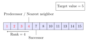
The above procedure only performs exact matches, finding the position of a target value. However, it is trivial to extend binary search to perform approximate matches because binary search operates on sorted arrays. For example, binary search can be used to compute, for a given value, its rank (the number of smaller elements), predecessor (next-smallest element), successor (next-largest element), and nearest neighbor. Range queries seeking the number of elements between two values can be performed with two rank queries.[11]
- Rank queries can be performed with the procedure for finding the leftmost element. The number of elements less than the target value is returned by the procedure.[11]
- Predecessor queries can be performed with rank queries. If the rank of the target value is r, its predecessor is r − 1.[12]
- For successor queries, the procedure for finding the rightmost element can be used. If the result of running the procedure for the target value is r, then the successor of the target value is r + 1.[12]
- The nearest neighbor of the target value is either its predecessor or successor, whichever is closer.
- Range queries are also straightforward.[12] Once the ranks of the two values are known, the number of elements greater than or equal to the first value and less than the second is the difference of the two ranks. This count can be adjusted up or down by one according to whether the endpoints of the range should be considered to be part of the range and whether the array contains keys matching those endpoints.[13]
Performance
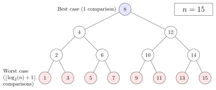
The performance of binary search can be analyzed by reducing the procedure to a binary comparison tree. The root node of the tree is the middle element of the array. The middle element of the lower half is the left child node of the root and the middle element of the upper half is the right child node of the root. The rest of the tree is built in a similar fashion. This model represents binary search. Starting from the root node, the left or right subtrees are traversed depending on whether the target value is less or more than the node under consideration. This represents the successive elimination of elements.[6][14]
In the worst case, binary search makes iterations of the comparison loop, where the notation denotes the floor function that yields the greatest integer less than or equal to the argument, and is the binary logarithm. The worst case is reached when the search reaches the deepest level of the tree. This is equivalent to a binary search that has reduced to one element and always eliminates the smaller subarray out of the two in each iteration if they are not of equal size.[lower-alpha 1][14]


The worst case may also be reached when the target element is not in the array. If is one less than a power of two, then this is always the case. Otherwise, the search may perform iterations if the search reaches the deepest level of the tree. However, it may make iterations, which is one less than the worst case, if the search ends at the second-deepest level of the tree.[15]


On average, assuming that each element is equally likely to be searched, binary search makes iterations when the target element is in the array. This is approximately equal to iterations. When the target element is not in the array, binary search makes iterations on average, assuming that the range between and outside elements is equally likely to be searched.[14]


In the best case, where the target value is the middle element of the array, its position is returned after one iteration.[16]
In terms of iterations, no search algorithm that works only by comparing elements can exhibit better average and worst-case performance than binary search. The comparison tree representing binary search has the fewest levels possible as every level above the lowest level of the tree is filled completely.[lower-alpha 2] Otherwise, the search algorithm can eliminate few elements in an iteration, increasing the number of iterations required in the average and worst case. This is the case for other search algorithms based on comparisons, as while they may work faster on some target values, the average performance over all elements is worse than binary search. By dividing the array in half, binary search ensures that the size of both subarrays are as similar as possible.[14]
Performance of alternative procedure
Each iteration of the binary search procedure defined above makes one or two comparisons, checking if the middle element is equal to the target in each iteration. Assuming that each element is equally likely to be searched, each iteration makes 1.5 comparisons on average. A variation of the algorithm checks whether the middle element is equal to the target at the end of the search. On average, this eliminates half a comparison from each iteration. This slightly cuts the time taken per iteration on most computers. However, it guarantees that the search takes the maximum number of iterations, on average adding one iteration to the search. Because the comparison loop is performed only times in the worst case, the slight increase in efficiency per iteration does not compensate for the extra iteration for all but enormous .[lower-alpha 3][17][18]
Binary search versus other schemes
Sorted arrays with binary search are a very inefficient solution when insertion and deletion operations are interleaved with retrieval, taking time for each such operation. In addition, sorted arrays can complicate memory use especially when elements are often inserted into the array.[19] There are other data structures that support much more efficient insertion and deletion. Binary search can be used to perform exact matching and set membership (determining whether a target value is in a collection of values). There are data structures that support faster exact matching and set membership. However, unlike many other searching schemes, binary search can be used for efficient approximate matching, usually performing such matches in time regardless of the type or structure of the values themselves.[20] In addition, there are some operations, like finding the smallest and largest element, that can be performed efficiently on a sorted array.[11]


Hashing
For implementing associative arrays, hash tables, a data structure that maps keys to records using a hash function, are generally faster than binary search on a sorted array of records.[21] Most hash table implementations require only amortized constant time on average.[lower-alpha 4][23] However, hashing is not useful for approximate matches, such as computing the next-smallest, next-largest, and nearest key, as the only information given on a failed search is that the target is not present in any record.[24] Binary search is ideal for such matches, performing them in logarithmic time. Binary search also supports approximate matches. Some operations, like finding the smallest and largest element, can be done efficiently on sorted arrays but not on hash tables.[20]
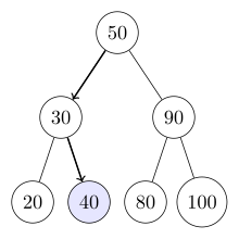
Trees
A binary search tree is a binary tree data structure that works based on the principle of binary search. The records of the tree are arranged in sorted order, and each record in the tree can be searched using an algorithm similar to binary search, taking on average logarithmic time. Insertion and deletion also require on average logarithmic time in binary search trees. This can be faster than the linear time insertion and deletion of sorted arrays, and binary trees retain the ability to perform all the operations possible on a sorted array, including range and approximate queries.[20][25]
However, binary search is usually more efficient for searching as binary search trees will most likely be imperfectly balanced, resulting in slightly worse performance than binary search. This even applies to balanced binary search trees, binary search trees that balance their own nodes, because they rarely produce optimally-balanced trees. Although unlikely, the tree may be severely imbalanced with few internal nodes with two children, resulting in the average and worst-case search time approaching comparisons.[lower-alpha 5] Binary search trees take more space than sorted arrays.[27]
Binary search trees lend themselves to fast searching in external memory stored in hard disks, as binary search trees can efficiently be structured in filesystems. The B-tree generalizes this method of tree organization. B-trees are frequently used to organize long-term storage such as databases and filesystems.[28][29]
Linear search
Linear search is a simple search algorithm that checks every record until it finds the target value. Linear search can be done on a linked list, which allows for faster insertion and deletion than an array. Binary search is faster than linear search for sorted arrays except if the array is short, although the array needs to be sorted beforehand.[lower-alpha 6][31] All sorting algorithms based on comparing elements, such as quicksort and merge sort, require at least comparisons in the worst case.[32] Unlike linear search, binary search can be used for efficient approximate matching. There are operations such as finding the smallest and largest element that can be done efficiently on a sorted array but not on an unsorted array.[33]

Set membership algorithms
A related problem to search is set membership. Any algorithm that does lookup, like binary search, can also be used for set membership. There are other algorithms that are more specifically suited for set membership. A bit array is the simplest, useful when the range of keys is limited. It compactly stores a collection of bits, with each bit representing a single key within the range of keys. Bit arrays are very fast, requiring only time.[34] The Judy1 type of Judy array handles 64-bit keys efficiently.[35]

For approximate results, Bloom filters, another probabilistic data structure based on hashing, store a set of keys by encoding the keys using a bit array and multiple hash functions. Bloom filters are much more space-efficient than bit arrays in most cases and not much slower: with hash functions, membership queries require only time. However, Bloom filters suffer from false positives.[lower-alpha 7][lower-alpha 8][37]


Other data structures
There exist data structures that may improve on binary search in some cases for both searching and other operations available for sorted arrays. For example, searches, approximate matches, and the operations available to sorted arrays can be performed more efficiently than binary search on specialized data structures such as van Emde Boas trees, fusion trees, tries, and bit arrays. These specialized data structures are usually only faster because they take advantage of the properties of keys with a certain attribute (usually keys that are small integers), and thus will be time or space consuming for keys that lack that attribute.[20] As long as the keys can be ordered, these operations can always be done at least efficiently on a sorted array regardless of the keys. Some structures, such as Judy arrays, use a combination of approaches to mitigate this while retaining efficiency and the ability to perform approximate matching.[35]
Variations
Uniform binary search
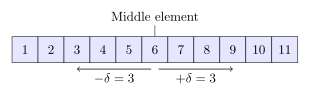
Uniform binary search stores, instead of the lower and upper bounds, the index of the middle element and the change in the middle element from the current iteration to the next iteration. Each step reduces the change by about half. For example, if the array to be searched is [1, 2, 3, 4, 5, 6, 7, 8, 9, 10, 11], the middle element would be 6. Uniform binary search works on the basis that the difference between the index of middle element of the array and the left and right subarrays is the same. In this case, the middle element of the left subarray ([1, 2, 3, 4, 5]) is 3 and the middle element of the right subarray ([7, 8, 9, 10, 11]) is 9. Uniform binary search would store the value of 3 as both indices differ from 6 by this same amount.[38] To reduce the search space, the algorithm either adds or subtracts this change from the middle element. The main advantage of uniform binary search is that the procedure can store a table of the differences between indices for each iteration of the procedure. Uniform binary search may be faster on systems where it is inefficient to calculate the midpoint, such as on decimal computers.[39]
Exponential search
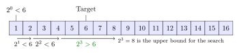
Exponential search extends binary search to unbounded lists. It starts by finding the first element with an index that is both a power of two and greater than the target value. Afterwards, it sets that index as the upper bound, and switches to binary search. A search takes iterations of the exponential search and at most iterations of the binary search, where is the position of the target value. Exponential search works on bounded lists, but becomes an improvement over binary search only if the target value lies near the beginning of the array.[40]


Interpolation search

Instead of calculating the midpoint, interpolation search estimates the position of the target value, taking into account the lowest and highest elements in the array as well as length of the array. This is only possible if the array elements are numbers. It works on the basis that the midpoint is not the best guess in many cases. For example, if the target value is close to the highest element in the array, it is likely to be located near the end of the array.[41] When the distribution of the array elements is uniform or near uniform, it makes comparisons.[41][42][43]

In practice, interpolation search is slower than binary search for small arrays, as interpolation search requires extra computation. Its time complexity grows more slowly than binary search, but this only compensates for the extra computation for large arrays.[41]
Fractional cascading

Fractional cascading is a technique that speeds up binary searches for the same element in multiple sorted arrays. Searching each array separately requires time, where is the number of arrays. Fractional cascading reduces this to by storing specific information in each array about each element and its position in the other arrays.[44][45]


Fractional cascading was originally developed to efficiently solve various computational geometry problems. Fractional cascading has been applied elsewhere, such as in data mining and Internet Protocol routing.[44]
Noisy binary search
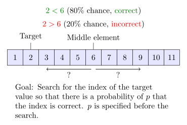
Noisy binary search algorithms solve the case where the algorithm cannot reliably compare elements of the array. For each pair of elements, there is a certain probability that the algorithm makes the wrong comparison. Noisy binary search can find the correct position of the target with a given probability that controls the reliability of the yielded position.[lower-alpha 9][lower-alpha 10][49][50]
Quantum binary search
Classical computers are bounded to the worst case of exactly iterations when performing binary search. Quantum algorithms for binary search are still bounded to a proportion of queries (representing iterations of the classical procedure), but the constant factor is less than one, providing for faster performance on quantum computers. Any exact quantum binary search procedure—that is, a procedure that always yields the correct result—requires at least queries in the worst case, where is the natural logarithm.[51] There is an exact quantum binary search procedure that runs in queries in the worst case.[52] In comparison, Grover's algorithm is the optimal quantum algorithm for searching an unordered list of elements, and it requires queries.[53]


History
In 1946, John Mauchly made the first mention of binary search as part of the Moore School Lectures, a seminal and foundational college course in computing.[9] In 1957, William Wesley Peterson published the first method for interpolation search.[9][54] Every published binary search algorithm worked only for arrays whose length is one less than a power of two[lower-alpha 11] until 1960, when Derrick Henry Lehmer published a binary search algorithm that worked on all arrays.[56] In 1962, Hermann Bottenbruch presented an ALGOL 60 implementation of binary search that placed the comparison for equality at the end, increasing the average number of iterations by one, but reducing to one the number of comparisons per iteration.[8] The uniform binary search was developed by A. K. Chandra of Stanford University in 1971.[9] In 1986, Bernard Chazelle and Leonidas J. Guibas introduced fractional cascading as a method to solve numerous search problems in computational geometry.[44][57][58]
Implementation issues
Although the basic idea of binary search is comparatively straightforward, the details can be surprisingly tricky ... — Donald Knuth[2]
When Jon Bentley assigned binary search as a problem in a course for professional programmers, he found that ninety percent failed to provide a correct solution after several hours of working on it, mainly because the incorrect implementations failed to run or returned a wrong answer in rare edge cases.[59] A study published in 1988 shows that accurate code for it is only found in five out of twenty textbooks.[60] Furthermore, Bentley's own implementation of binary search, published in his 1986 book Programming Pearls, contained an overflow error that remained undetected for over twenty years. The Java programming language library implementation of binary search had the same overflow bug for more than nine years.[61]
In a practical implementation, the variables used to represent the indices will often be of fixed size, and this can result in an arithmetic overflow for very large arrays. If the midpoint of the span is calculated as (L + R) / 2, then the value of L + R may exceed the range of integers of the data type used to store the midpoint, even if L and R are within the range. If L and R are nonnegative, this can be avoided by calculating the midpoint as L + (R − L) / 2.[62]
If the target value is greater than the greatest value in the array, and the last index of the array is the maximum representable value of L, the value of L will eventually become too large and overflow. A similar problem will occur if the target value is smaller than the least value in the array and the first index of the array is the smallest representable value of R. In particular, this means that R must not be an unsigned type if the array starts with index 0.[60][62]
An infinite loop may occur if the exit conditions for the loop are not defined correctly. Once L exceeds R, the search has failed and must convey the failure of the search. In addition, the loop must be exited when the target element is found, or in the case of an implementation where this check is moved to the end, checks for whether the search was successful or failed at the end must be in place. Bentley found that most of the programmers who incorrectly implemented binary search made an error in defining the exit conditions.[8][63]
Library support
Many languages' standard libraries include binary search routines:
- C provides the function
bsearch()in its standard library, which is typically implemented via binary search, although the official standard does not require it so.[64] - C++'s Standard Template Library provides the functions
binary_search(),lower_bound(),upper_bound()andequal_range().[65] - COBOL provides the
SEARCH ALLverb for performing binary searches on COBOL ordered tables.[66] - Go's
sortstandard library package contains the functionsSearch,SearchInts,SearchFloat64s, andSearchStrings, which implement general binary search, as well as specific implementations for searching slices of integers, floating-point numbers, and strings, respectively.[67] - Java offers a set of overloaded
binarySearch()static methods in the classesArraysandCollectionsin the standardjava.utilpackage for performing binary searches on Java arrays and onLists, respectively.[68][69] - Microsoft's .NET Framework 2.0 offers static generic versions of the binary search algorithm in its collection base classes. An example would be
System.Array's methodBinarySearch<T>(T[] array, T value).[70] - For Objective-C, the Cocoa framework provides the
NSArray -indexOfObject:inSortedRange:options:usingComparator:method in Mac OS X 10.6+.[71] Apple's Core Foundation C framework also contains aCFArrayBSearchValues()function.[72] - Python provides the
bisectmodule.[73] - Ruby's Array class includes a
bsearchmethod with built-in approximate matching.[74]
See also
- Bisection method – the same idea used to solve equations in the real numbers
- Multiplicative binary search - binary search variation with simplified midpoint calculation
Notes and references
Notes
- ↑ This happens as binary search will not always divide the array perfectly. Take for example the array [1, 2, ..., 16]. The first iteration will select the midpoint of 8. On the left subarray are eight elements, but on the right are nine. If the search takes the right path, there is a higher chance that the search will make the maximum number of comparisons.[14]
- ↑ Any search algorithm based solely on comparisons can be represented using a binary comparison tree. An internal path is any path from the root to an existing node. Let be the internal path length, the sum of the lengths of all internal paths. If each element is equally likely to be searched, the average case is or simply one plus the average of all the internal path lengths of the tree. This is because internal paths represent the elements that the search algorithm compares to the target. The lengths of these internal paths represent the number of iterations after the root node. Adding the average of these lengths to the one iteration at the root yields the average case. Therefore, to minimize the average number of comparisons, the internal path length must be minimized. It turns out that the tree for binary search minimizes the internal path length. Knuth 1998 proved that the external path length (the path length over all nodes where both children are present for each already-existing node) is minimized when the external nodes (the nodes with no children) lie within two consecutive levels of the tree. This also applies to internal paths as internal path length is linearly related to external path length . For any tree of nodes, . When each subtree has a similar number of nodes, or equivalently the array is divided into halves in each iteration, the external nodes as well as their interior parent nodes lie within two levels. It follows that binary search minimizes the number of average comparisons as its comparison tree has the lowest possible internal path length.[14]
- ↑ Knuth 1998 showed on his MIX computer model, intended to represent an ordinary computer, that the average running time of this variation for a successful search is units of time compared to units for regular binary search. The time complexity for this variation grows slightly more slowly, but at the cost of higher initial complexity. [17]
- ↑ It is possible to perform hashing in guaranteed constant time.[22]
- ↑ The worst binary search tree for searching can be produced by inserting the values in sorted order or in an alternating lowest-highest key pattern.[26]
- ↑ Knuth 1998 performed a formal time performance analysis of both of these search algorithms. On Knuth's MIX computer, which Knuth designed as a representation of an ordinary computer, binary search takes on average units of time for a successful search, while linear search with a sentinel node at the end of the list takes units. Linear search has lower initial complexity because it requires minimal computation, but it quickly outgrows binary search in complexity. On the MIX computer, binary search only outperforms linear search with a sentinel if .[14][30]
- ↑ This is because simply setting all of the bits which the hash functions point to for a specific key can affect queries for other keys which have a common hash location for one or more of the functions.[36]
- ↑ There exist improvements of the Bloom filter which improve on its complexity or support deletion; for example, the cuckoo filter exploits cuckoo hashing to gain these advantages.[36]
- ↑ Using noisy comparisons, Ben-Or & Hassidim 2008 established that any noisy binary search procedure must make at least comparisons on average, where is the binary entropy function and is the probability that the procedure yields the wrong position.[46]
- ↑ The noisy binary search problem can be considered as a case of the Rényi-Ulam game,[47] a variant of Twenty Questions where the answers may be wrong.[48]
- ↑ That is, arrays of length 1, 3, 7, 15, 31 ...[55]


Citations
- ↑ Willams, Jr., Louis F. (22 April 1976). A modification to the half-interval search (binary search) method. Proceedings of the 14th ACM Southeast Conference. ACM. pp. 95–101. doi:10.1145/503561.503582. Retrieved 29 June 2018.
- 1 2 Knuth 1998, §6.2.1 ("Searching an ordered table"), subsection "Binary search".
- ↑ Butterfield & Ngondi 2016, p. 46.
- ↑ Cormen et al. 2009, p. 39.
- ↑ Weisstein, Eric W. "Binary search". MathWorld.
- 1 2 Flores, Ivan; Madpis, George (1 September 1971). "Average binary search length for dense ordered lists". Communications of the ACM. 14 (9): 602–603. doi:10.1145/362663.362752. ISSN 0001-0782. Retrieved 29 June 2018.
- 1 2 3 Knuth 1998, §6.2.1 ("Searching an ordered table"), subsection "Algorithm B".
- 1 2 3 4 Bottenbruch, Hermann (1 April 1962). "Structure and use of ALGOL 60". Journal of the ACM. 9 (2): 161–221. doi:10.1145/321119.321120. ISSN 0004-5411. Retrieved 30 June 2018. Procedure is described at p. 214 (§43), titled "Program for Binary Search".
- 1 2 3 4 5 Knuth 1998, §6.2.1 ("Searching an ordered table"), subsection "History and bibliography".
- 1 2 Kasahara & Morishita 2006, pp. 8–9.
- 1 2 3 Sedgewick & Wayne 2011, §3.1, subsection "Rank and selection".
- 1 2 3 Goldman & Goldman 2008, pp. 461–463.
- ↑ Sedgewick & Wayne 2011, §3.1, subsection "Range queries".
- 1 2 3 4 5 6 7 Knuth 1998, §6.2.1 ("Searching an ordered table"), subsection "Further analysis of binary search".
- ↑ Knuth 1998, §6.2.1 ("Searching an ordered table"), "Theorem B".
- ↑ Chang 2003, p. 169.
- 1 2 Knuth 1998, §6.2.1 ("Searching an ordered table"), subsection "Exercise 23".
- ↑ Rolfe, Timothy J. (1997). "Analytic derivation of comparisons in binary search". ACM SIGNUM Newsletter. 32 (4): 15–19. doi:10.1145/289251.289255.
- ↑ Knuth 1997, §2.2.2 ("Sequential Allocation").
- 1 2 3 4 Beame, Paul; Fich, Faith E. (2001). "Optimal bounds for the predecessor problem and related problems". Journal of Computer and System Sciences. 65 (1): 38–72. doi:10.1006/jcss.2002.1822.

- ↑ Knuth 1998, §6.4 ("Hashing").
- ↑ Knuth 1998, §6.4 ("Hashing"), subsection "History".
- ↑ Dietzfelbinger, Martin; Karlin, Anna; Mehlhorn, Kurt; Meyer auf der Heide, Friedhelm; Rohnert, Hans; Tarjan, Robert E. (August 1994). "Dynamic perfect hashing: upper and lower bounds". SIAM Journal on Computing. 23 (4): 738–761. doi:10.1137/S0097539791194094.
- ↑ Morin, Pat. "Hash tables" (PDF). p. 1. Retrieved 28 March 2016.
- ↑ Sedgewick & Wayne 2011, §3.2 ("Binary Search Trees"), subsection "Order-based methods and deletion".
- ↑ Knuth 1998, §6.2.2 ("Binary tree searching"), subsection "But what about the worst case?".
- ↑ Sedgewick & Wayne 2011, §3.5 ("Applications"), "Which symbol-table implementation should I use?".
- ↑ Knuth 1998, §5.4.9 ("Disks and Drums").
- ↑ Knuth 1998, §6.2.4 ("Multiway trees").
- ↑ Knuth 1998, Answers to Exercises (§6.2.1) for "Exercise 5".
- ↑ Knuth 1998, §6.2.1 ("Searching an ordered table").
- ↑ Knuth 1998, §5.3.1 ("Minimum-Comparison sorting").
- ↑ Sedgewick & Wayne 2011, §3.2 ("Ordered symbol tables").
- ↑ Knuth 2011, §7.1.3 ("Bitwise Tricks and Techniques").
- 1 2 Silverstein, Alan, Judy IV shop manual (PDF), Hewlett-Packard, pp. 80&ndash, 81
- 1 2 Fan, Bin; Andersen, Dave G.; Kaminsky, Michael; Mitzenmacher, Michael D. (2014). Cuckoo filter: practically better than Bloom. Proceedings of the 10th ACM International on Conference on Emerging Networking Experiments and Technologies. pp. 75–88. doi:10.1145/2674005.2674994.
- ↑ Bloom, Burton H. (1970). "Space/time trade-offs in hash coding with allowable errors" (PDF). Communications of the ACM. 13 (7): 422–426. doi:10.1145/362686.362692. Archived from the original (PDF) on 4 November 2004. Retrieved 26 October 2017.
- ↑ Knuth 1998, §6.2.1 ("Searching an ordered table"), subsection "An important variation".
- ↑ Knuth 1998, §6.2.1 ("Searching an ordered table"), subsection "Algorithm U".
- ↑ Moffat & Turpin 2002, p. 33.
- 1 2 3 Knuth 1998, §6.2.1 ("Searching an ordered table"), subsection "Interpolation search".
- ↑ Knuth 1998, §6.2.1 ("Searching an ordered table"), subsection "Exercise 22".
- ↑ Perl, Yehoshua; Itai, Alon; Avni, Haim (1978). "Interpolation search—a log log n search". Communications of the ACM. 21 (7): 550–553. doi:10.1145/359545.359557.
- 1 2 3 Chazelle, Bernard; Liu, Ding (6 July 2001). Lower bounds for intersection searching and fractional cascading in higher dimension. 33rd ACM Symposium on Theory of Computing. ACM. pp. 322–329. doi:10.1145/380752.380818. ISBN 978-1-58113-349-3. Retrieved 30 June 2018.
- ↑ Chazelle, Bernard; Liu, Ding (1 March 2004). "Lower bounds for intersection searching and fractional cascading in higher dimension" (PDF). Journal of Computer and System Sciences. 68 (2): 269–284. doi:10.1016/j.jcss.2003.07.003. ISSN 0022-0000. Retrieved 30 June 2018.
- ↑ Ben-Or, Michael; Hassidim, Avinatan (2008). "The Bayesian learner is optimal for noisy binary search (and pretty good for quantum as well)" (PDF). 49th Symposium on Foundations of Computer Science. pp. 221–230. doi:10.1109/FOCS.2008.58. ISBN 978-0-7695-3436-7.
- ↑ Pelc, Andrzej (2002). "Searching games with errors—fifty years of coping with liars". Theoretical Computer Science. 270 (1–2): 71–109. doi:10.1016/S0304-3975(01)00303-6.
- ↑ Rényi, Alfréd (1961). "On a problem in information theory". Magyar Tudományos Akadémia Matematikai Kutató Intézetének Közleményei (in Hungarian). 6: 505–516. MR 0143666.
- ↑ Pelc, Andrzej (1989). "Searching with known error probability". Theoretical Computer Science. 63 (2): 185–202. doi:10.1016/0304-3975(89)90077-7.
- ↑ Rivest, Ronald L.; Meyer, Albert R.; Kleitman, Daniel J.; Winklmann, K. Coping with errors in binary search procedures. 10th ACM Symposium on Theory of Computing. doi:10.1145/800133.804351.
- ↑ Høyer, Peter; Neerbek, Jan; Shi, Yaoyun (2002). "Quantum complexities of ordered searching, sorting, and element distinctness". Algorithmica. 34 (4): 429–448. arXiv:quant-ph/0102078. doi:10.1007/s00453-002-0976-3.
- ↑ Childs, Andrew M.; Landahl, Andrew J.; Parrilo, Pablo A. (2007). "Quantum algorithms for the ordered search problem via semidefinite programming". Physical Review A. 75 (3). 032335. arXiv:quant-ph/0608161. Bibcode:2007PhRvA..75c2335C. doi:10.1103/PhysRevA.75.032335.
- ↑ Grover, Lov K. (1996). A fast quantum mechanical algorithm for database search. 28th ACM Symposium on Theory of Computing. Philadelphia, PA. pp. 212–219. arXiv:quant-ph/9605043. doi:10.1145/237814.237866.
- ↑ Peterson, William Wesley (1957). "Addressing for random-access storage". IBM Journal of Research and Development. 1 (2): 130–146. doi:10.1147/rd.12.0130.
- ↑ "2n−1". OEIS A000225. Retrieved 7 May 2016.
- ↑ Lehmer, Derrick (1960). Teaching combinatorial tricks to a computer. Proceedings of Symposia in Applied Mathematics. 10. pp. 180–181. doi:10.1090/psapm/010.
- ↑ Chazelle, Bernard; Guibas, Leonidas J. (1986). "Fractional cascading: I. A data structuring technique" (PDF). Algorithmica. 1 (1): 133–162. doi:10.1007/BF01840440.
- ↑ Chazelle, Bernard; Guibas, Leonidas J. (1986), "Fractional cascading: II. Applications" (PDF), Algorithmica, 1 (1): 163–191, doi:10.1007/BF01840441
- ↑ Bentley 2000, §4.1 ("The Challenge of Binary Search").
- 1 2 Pattis, Richard E. (1988). "Textbook errors in binary searching". SIGCSE Bulletin. 20: 190–194. doi:10.1145/52965.53012.
- ↑ Bloch, Joshua (2 June 2006). "Extra, extra – read all about it: nearly all binary searches and mergesorts are broken". Google Research Blog. Retrieved 21 April 2016.
- 1 2 Ruggieri, Salvatore (2003). "On computing the semi-sum of two integers" (PDF). Information Processing Letters. 87 (2): 67–71. doi:10.1016/S0020-0190(03)00263-1.
- ↑ Bentley 2000, §4.4 ("Principles").
- ↑ "bsearch – binary search a sorted table". The Open Group Base Specifications (7th ed.). The Open Group. 2013. Retrieved 28 March 2016.
- ↑ Stroustrup 2013, p. 945.
- ↑ Unisys (2012), COBOL ANSI-85 programming reference manual, 1, pp. 598–601
- ↑ "Package sort". The Go Programming Language. Retrieved 28 April 2016.
- ↑ "java.util.Arrays". Java Platform Standard Edition 8 Documentation. Oracle Corporation. Retrieved 1 May 2016.
- ↑ "java.util.Collections". Java Platform Standard Edition 8 Documentation. Oracle Corporation. Retrieved 1 May 2016.
- ↑ "List<T>.BinarySearch method (T)". Microsoft Developer Network. Retrieved 10 April 2016.
- ↑ "NSArray". Mac Developer Library. Apple Inc. Retrieved 1 May 2016.
- ↑ "CFArray". Mac Developer Library. Apple Inc. Retrieved 1 May 2016.
- ↑ "8.6. bisect — Array bisection algorithm". The Python Standard Library. Python Software Foundation. Retrieved 26 March 2018.
- ↑ Fitzgerald 2007, p. 152.
Works
- Bentley, Jon (2000). Programming pearls (2nd ed.). Addison-Wesley. ISBN 978-0-201-65788-3.
- Butterfield, Andrew; Ngondi, Gerard E. (2016). A dictionary of computer science (7th ed.). Oxford, UK: Oxford University Press. ISBN 978-0-19-968897-5.
- Chang, Shi-Kuo (2003). Data structures and algorithms. Software Engineering and Knowledge Engineering. 13. Singapore: World Scientific. ISBN 978-981-238-348-8.
- Cormen, Thomas H.; Leiserson, Charles E.; Rivest, Ronald L.; Stein, Clifford (2009). Introduction to algorithms (3rd ed.). MIT Press and McGraw-Hill. ISBN 978-0-262-03384-8.
- Fitzgerald, Michael (2007). Ruby pocket reference. Sebastopol, California: O'Reilly Media. ISBN 978-1-4919-2601-7.
- Goldman, Sally A.; Goldman, Kenneth J. (2008). A practical guide to data structures and algorithms using Java. Boca Raton, Florida: CRC Press. ISBN 978-1-58488-455-2.
- Kasahara, Masahiro; Morishita, Shinichi (2006). Large-scale genome sequence processing. London, UK: Imperial College Press. ISBN 978-1-86094-635-6.
- Knuth, Donald (1997). Fundamental algorithms. The Art of Computer Programming. 1 (3rd ed.). Reading, MA: Addison-Wesley Professional. ISBN 978-0-201-89683-1.
- Knuth, Donald (1998). Sorting and searching. The Art of Computer Programming. 3 (2nd ed.). Reading, MA: Addison-Wesley Professional. ISBN 978-0-201-89685-5.
- Knuth, Donald (2011). Combinatorial algorithms. The Art of Computer Programming. 4A (1st ed.). Reading, MA: Addison-Wesley Professional. ISBN 978-0-201-03804-0.
- Moffat, Alistair; Turpin, Andrew (2002). Compression and coding algorithms. Hamburg, Germany: Kluwer Academic Publishers. doi:10.1007/978-1-4615-0935-6. ISBN 978-0-7923-7668-2.
- Sedgewick, Robert; Wayne, Kevin (2011). Algorithms (4th ed.). Upper Saddle River, New Jersey: Addison-Wesley Professional. ISBN 978-0-321-57351-3.
Condensed web version:

- Stroustrup, Bjarne (2013). The C++ programming language (4th ed.). Upper Saddle River, New Jersey: Addison-Wesley Professional. ISBN 978-0-321-56384-2.
External links
| The Wikibook Algorithm implementation has a page on the topic of: Binary search |