Angular velocity

In physics, the angular velocity of a particle is the rate at which it rotates around a chosen center point: that is, the time rate of change of its angular displacement relative to the origin (i.e. in layman's terms: how quickly an object goes around something over a period of time - e.g. how fast the earth orbits the sun). It is measured in angle per unit time, radians per second in SI units, and is usually represented by the symbol omega (ω, sometimes Ω). By convention, positive angular velocity indicates counter-clockwise rotation, while negative is clockwise.

For example, a geostationary satellite completes one orbit per day above the equator, or 360 degrees per 24 hours, and has angular velocity ω = 360 / 24 = 15 degrees per hour, or 2π / 24 ≈ 0.26 radians per hour. If angle is measured in radians, the linear velocity is the radius times the angular velocity, $v=r\omega$ . With orbital radius 42,000 km from the earth's center, the satellite's speed through space is thus v = 42,000 × 0.26 ≈ 11,000 km/hr. The angular velocity is positive since the satellite travels eastward with the Earth's rotation (counter-clockwise from above the north pole.)

In three dimensions, angular velocity is a pseudovector, with its magnitude measuring the rate of rotation, and its direction pointing along the axis of rotation (perpendicular to the radius and velocity vectors). The up-or-down orientation of angular velocity is conventionally specified by the right-hand rule.^[1]

Angular velocity of a particle

Particle in two dimensions

The angular velocity of the particle at P with respect to the origin O is determined by the perpendicular component of the velocity vector v.

In the simplest case of circular motion at radius r, with position given by the angular displacement $\phi (t)$ from the x-axis, the angular velocity is the rate of change of angle with respect to time: $\omega ={\tfrac {d\phi }{dt}}$ . If $\phi$ is measured in radians, the distance from the x-axis around the circle to the particle is $\ell =r\phi$ , and the linear velocity is $v(t)={\tfrac {d\ell }{dt}}=r\omega (t)$ , so that $\omega ={\tfrac {v}{r}}$ .

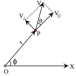
In the general case of a particle moving in the plane, the angular velocity is measured relative to a chosen center point, called the origin. The diagram shows the radius vector r from the origin O to the particle P, with its polar coordinates $(r,\phi )$ . (All variables are functions of time t.) The particle has linear velocity splitting as ${\mathbf {v}}={\mathbf {v}}_{\|}+{\mathbf {v}}_{\perp }$ , with the radial component ${\mathbf {v}}_{\|}$ parallel to the radius, and the cross-radial (or tangential or circular) component ${\mathbf {v}}_{\perp }$ perpendicular to the radius. When there is no radial component, the particle moves around the origin in a circle; but when there is no cross-radial component, it moves in a straight line from the origin. Since radial motion leaves the angle unchanged, only the cross-radial component of linear velocity contributes to angular velocity.

The angular velocity ω is the rate of change of angle with respect to time, which can be computed from the cross-radial velocity as:

\omega ={\frac {d\phi }{dt}}={\frac {v_{\perp }}{r}}.

Here the cross-radial speed $v_\perp$ is the signed magnitude of ${\mathbf {v}}_{\perp }$ , positive for counter-clockwise motion, negative for clockwise. Taking polar coordinates for the linear velocity v gives magnitude v (linear speed) and angle θ relative to the radius vector; in these terms, $v_{\perp }=v\sin(\theta )$ , so that

\omega ={\frac {v\sin(\theta )}{r}}.

These formulas may be derived from ${\mathbf {r}}=(x(t),y(t))$ , ${\mathbf {v}}=(x'(t),y'(t))$ and $\phi =\arctan(y(t)/x(t))$ , together with the projection formula $v_{\perp }={\tfrac {{\mathbf {r}}^{\perp }\!\!}{r}}\cdot {\mathbf {v}}$ , where ${\mathbf {r}}^{\perp }=(-y,x)$ .

In two dimensions, angular velocity is a number with plus or minus sign indicating orientation, but not pointing in a direction. The sign is conventionally taken to be positive if the radius vector turns counter-clockwise, and negative if clockwise. Angular velocity may be termed a pseudoscalar, a numerical quantity which changes sign under a parity inversion, such as inverting one axis or switching the two axes.

Particle in three dimensions

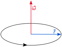
The angular velocity describes the rate of change of angular position, and the instantaneous axis of rotation. In this case (counter-clockwise rotation) the vector points up.

In three-dimensional space, we again have the position vector r of a moving particle, its radius vector from the origin. Angular velocity is a vector (or pseudovector) whose magnitude measures the rate at which the radius sweeps out angle, and whose direction shows the principal axis of rotation. Its up-or-down direction is given by the right-hand rule.

Let the axial vector $\bold{u}$ be the unit-length vector perpendicular to the plane of rotation spanned by the radius and velocity vectors, so that the direction of rotation is counter-clockwise looking from the top of $\bold{u}$ . Taking polar coordinates $(r,\phi )$ in the plane of rotation, as in the two-dimensional case above, one may define the angular velocity vector as:

{\boldsymbol {\omega }}=\omega {\mathbf {u}}={\tfrac {d\phi }{dt}}{\mathbf {u}}={\frac {v\sin(\theta )}{r}}{\mathbf {u}},

where θ is the angle between r and v. In terms of the cross product, this is:

{\boldsymbol {\omega }}={\frac {{\mathbf {r}}\times {\mathbf {v}}}{r^{2}}}.

From this, one can recover the tangential velocity as:

{\mathbf {v}}_{\perp }={\boldsymbol {\omega }}\times {\mathbf {r}}

Addition of angular velocity vectors

If a point rotates with angular velocity $\omega _{1}$ in a coordinate frame $F_{1}$ which itself rotates with an angular velocity $\omega _{2}$ with respect to an external frame $F_{2}$ , we can define $\omega_1 + \omega_2$ to be the composite angular velocity vector of the point with respect to $F_{2}$ . This operation coincides with usual addition of vectors, and it gives angular velocity the algebraic structure of a true vector, rather than just a pseudo-vector.

The only non-obvious property of the above addition is commutativity. This can be proven from the fact that the velocity tensor W (see below) is skew-symmetric, so that $R=e^{Wt}$ is a rotation matrix which can be expanded as $R=I+W\cdot dt+{\tfrac {1}{2}}(W\cdot dt)^{2}+\ldots$ . The composition of rotations is not commutative, but $(I+W_1\cdot dt)(I+W_2 \cdot dt)=(I+W_2 \cdot dt)(I+W_1\cdot dt)$ is commutative to first order, and therefore $\omega _{1}+\omega _{2}=\omega _{2}+\omega _{1}$ .

Angular velocity vector for a frame

Schematic construction for addition of angular velocity vectors for rotating frames

Given a rotating frame of three unit coordinate vectors, all the three must have the same angular speed at each instant. In such a frame, each vector may be considered as a moving particle with constant scalar radius.

The rotating frame appears in the context of rigid bodies, and special tools have been developed for it: the angular velocity may be described as a vector or equivalently as a tensor.

Consistent with the general definition, the angular velocity of a frame is defined as the angular velocity of any of the three vectors (same for all). The addition of angular velocity vectors for frames is also defined by the usual vector addition (composition of linear movements), and can be useful to decompose the rotation as in a gimbal. Components of the vector can be calculated as derivatives of the parameters defining the moving frames (Euler angles or rotation matrices). As in the general case, addition is commutative: $\omega _{1}+\omega _{2}=\omega _{2}+\omega _{1}$ .

By Euler's rotation theorem, any rotating frame possesses an instantaneous axis of rotation, which is the direction of the angular velocity vector, and the magnitude of the angular velocity is consistent with the two dimensional case.

Components from the vectors of the frame

Considering a coordinate vector of the frame as a particle, ${\mathbf {r}}={\mathbf {e}}_{i}$ with $|{\mathbf {e}}_{i}|=1$ , we obtain the angular velocity vector:

{\boldsymbol {\omega }}={\frac {\mathbf {r} \times \mathbf {v} }{r^{2}}}=\mathbf {e} _{1}\times {\dot {\mathbf {e} }}_{1}=\mathbf {e} _{2}\times {\dot {\mathbf {e} }}_{2}=\mathbf {e} _{3}\times {\dot {\mathbf {e} }}_{3}.

Here ${\mathbf {e}}_{i}$ are the columns of the matrix of the frame, and ${\dot {\mathbf {e}}}_{i}$ their time derivatives.

Components from Euler angles

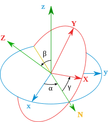
Diagram showing Euler frame in green

The components of the angular velocity pseudovector were first calculated by Leonhard Euler using his Euler angles and the use of an intermediate frame:

One axis of the reference frame (the precession axis)
The line of nodes of the moving frame with respect to the reference frame (nutation axis)
One axis of the moving frame (the intrinsic rotation axis)

Euler proved that the projections of the angular velocity pseudovector on each of these three axes is the derivative of its associated angle (which is equivalent to decomposing the instantaneous rotation into three instantaneous Euler rotations). Therefore:^[2]

{\boldsymbol \omega }={\dot \alpha }{\mathbf u}_{1}+{\dot \beta }{\mathbf u}_{2}+{\dot \gamma }{\mathbf u}_{3}

This basis is not orthonormal and it is difficult to use, but now the velocity vector can be changed to the fixed frame or to the moving frame with just a change of bases. For example, changing to the mobile frame:

{\boldsymbol {\omega }}=({\dot {\alpha }}\sin \beta \sin \gamma +{\dot {\beta }}\cos \gamma ){\mathbf {i}}+({\dot {\alpha }}\sin \beta \cos \gamma -{\dot {\beta }}\sin \gamma ){\mathbf {j}}+({\dot {\alpha }}\cos \beta +{\dot {\gamma }}){\mathbf {k}}

where ${\mathbf {i}},{\mathbf {j}},{\mathbf {k}}$ are unit vectors for the frame fixed in the moving body. This example has been made using the Z-X-Z convention for Euler angles.^[3]

Angular velocity tensor

The angular velocity vector ${\boldsymbol {\omega }}=(\omega _{x},\omega _{y},\omega _{z})$ defined above may be equivalently expressed as an angular velocity tensor, the matrix (or linear mapping) W = W(t) defined by:

W={\begin{pmatrix}0&-\omega _{z}&\omega _{y}\\\omega _{z}&0&-\omega _{x}\\-\omega _{y}&\omega _{x}&0\\\end{pmatrix}}

This is an infinitesimal rotation matrix. The linear mapping W acts as $({\boldsymbol {\omega }}\times )$ :

{\boldsymbol {\omega }}\times {\mathbf {r}}=W\cdot {\mathbf {r}}.

Calculation from the orientation matrix

A vector ${\mathbf {r}}$ undergoing uniform circular motion around an axis satisfies:

{\frac {d{\mathbf {r}}}{dt}}={\boldsymbol {\omega }}\times {\mathbf {r}}=W\cdot {\mathbf {r}}

Given the orientation matrix A(t) of a frame, whose columns are the moving orthonormal coordinate vectors ${\mathbf {e}}_{1},{\mathbf {e}}_{2},{\mathbf {e}}_{3}$ , we can obtain its angular velocity tensor W(t) as follows. Angular velocity must be the same for the three vectors ${\mathbf {r}}={\mathbf {e}}_{i}$ , so arranging the three vector equations into columns of a matrix, we have:

{\frac {dA}{dt}}=W\cdot A.

(This holds even if A(t) does not rotate uniformly.) Therefore the angular velocity tensor is:

W={\frac {dA}{dt}}\cdot A^{-1}={\frac {dA}{dt}}\cdot A^{\mathrm {T} },

since the inverse of the orthogonal matrix $A$ is its transpose $A^{\mathrm {T} }$ .

Properties of angular velocity tensors

In general, the angular velocity in an n-dimensional space is the time derivative of the angular displacement tensor, which is a second rank skew-symmetric tensor.

This tensor W will have n(n−1)/2 independent components, which is the dimension of the Lie algebra of the Lie group of rotations of an n-dimensional inner product space.^[4]

Duality with respect to the velocity vector

In three dimensions, angular velocity can be represented by a pseudovector because second rank tensors are dual to pseudovectors in three dimensions. Since the angular velocity tensor W = W(t) is a skew-symmetric matrix:

W={\begin{pmatrix}0&-\omega _{z}&\omega _{y}\\\omega _{z}&0&-\omega _{x}\\-\omega _{y}&\omega _{x}&0\\\end{pmatrix}},

its Hodge dual is a vector, which is precisely the previous angular velocity vector $\boldsymbol\omega=[\omega_x,\omega_y,\omega_z]$ .

Exponential of W

If we know an initial frame A(0) and we are given a constant angular velocity tensor W, we can obtain A(t) for any given t. Recall the matrix differential equation:

{\frac {dA}{dt}}=W\cdot A.

This equation can be integrated to give:

A(t)=e^{Wt}A(0),

which shows a connection with the Lie group of rotations.

W is skew-symmetric

We prove that angular velocity tensor is skew symmetric, i.e. $W={\frac {dA(t)}{dt}}\cdot A^{\text{T}}$ satisfies $W^{\text{T}}=-W$ .

A rotation matrix A is orthogonal, inverse to its transpose, so we have $I=A\cdot A^{\text{T}}$ . For $A=A(t)$ a frame matrix, taking the time derivative of the equation gives:

0={\frac {dA}{dt}}A^{\text{T}}+A{\frac {dA^{\text{T}}}{dt}}

Applying the formula $(AB)^{\text{T}}=B^{\text{T}}A^{\text{T}}$ ,

0={\frac {dA}{dt}}A^{\text{T}}+\left({\frac {dA}{dt}}A^{\text{T}}\right)^{\text{T}}=W+W^{\text{T}}

Thus, W is the negative of its transpose, which implies it is skew symmetric.

Coordinate-free description

At any instant $t$ , the angular velocity tensor represents a linear map between the position vector ${\mathbf {r}}(t)$ and the velocity vectors $\mathbf {v} (t)$ of a point on a rigid body rotating around the origin:

\mathbf {v} =W\mathbf {r} .

The relation between this linear map and the angular velocity pseudovector $\omega$ is the following.

Because W is the derivative of an orthogonal transformation, the bilinear form

B(\mathbf{r},\mathbf{s}) = (W\mathbf{r}) \cdot \mathbf{s}

is skew-symmetric. Thus we can apply the fact of exterior algebra that there is a unique linear form $L$ on $\Lambda ^{2}V$ that

L(\mathbf{r}\wedge \mathbf{s}) = B(\mathbf{r},\mathbf{s})

where $\mathbf {r} \wedge \mathbf {s} \in \Lambda ^{2}V$ is the exterior product of $\mathbf {r}$ and $\mathbf {s}$ .

Taking the sharp L^♯ of L we get

(W\mathbf {r} )\cdot \mathbf {s} =L^{\sharp }\cdot (\mathbf {r} \wedge \mathbf {s} )

Introducing $\omega :={\star }(L^{\sharp })$ , as the Hodge dual of L^♯, and applying the definition of the Hodge dual twice supposing that the preferred unit 3-vector is $\star 1$

(W\mathbf {r} )\cdot \mathbf {s} ={\star }({\star }(L^{\sharp })\wedge \mathbf {r} \wedge \mathbf {s} )={\star }(\omega \wedge \mathbf {r} \wedge \mathbf {s} )={\star }(\omega \wedge \mathbf {r} )\cdot \mathbf {s} =(\omega \times \mathbf {r} )\cdot \mathbf {s} ,

where

\omega \times \mathbf {r} :={\star }(\omega \wedge \mathbf {r} )

by definition.

Because $\mathbf {s}$ is an arbitrary vector, from nondegeneracy of scalar product follows

W\mathbf{r} = \omega \times \mathbf{r}

Angular velocity as a vector field

For angular velocity tensor maps positions to velocities, it is a vector field. In particular, this vector field is a Killing vector field belonging to an element of the Lie algebra so(3) of the 3-dimensional rotation group SO(3). This element of so(3) can also be regarded as the angular velocity vector.

Rigid body considerations

Position of point P located in the rigid body (shown in blue). R_i is the position with respect to the lab frame, centered at O and r_i is the position with respect to the rigid body frame, centered at O′. The origin of the rigid body frame is at vector position R from the lab frame.

The same equations for the angular speed can be obtained reasoning over a rotating rigid body. Here is not assumed that the rigid body rotates around the origin. Instead, it can be supposed rotating around an arbitrary point that is moving with a linear velocity V(t) in each instant.

To obtain the equations, it is convenient to imagine a rigid body attached to the frames and consider a coordinate system that is fixed with respect to the rigid body. Then we will study the coordinate transformations between this coordinate and the fixed "laboratory" system.

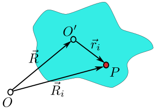
As shown in the figure on the right, the lab system's origin is at point O, the rigid body system origin is at O′ and the vector from O to O′ is R. A particle (i) in the rigid body is located at point P and the vector position of this particle is R_i in the lab frame, and at position r_i in the body frame. It is seen that the position of the particle can be written:

\mathbf{R}_i=\mathbf{R}+\mathbf{r}_i

The defining characteristic of a rigid body is that the distance between any two points in a rigid body is unchanging in time. This means that the length of the vector $\mathbf {r} _{i}$ is unchanging. By Euler's rotation theorem, we may replace the vector $\mathbf {r} _{i}$ with $\mathcal{R}\mathbf{r}_{io}$ where ${\mathcal {R}}$ is a 3×3 rotation matrix and $\mathbf{r}_{io}$ is the position of the particle at some fixed point in time, say t = 0. This replacement is useful, because now it is only the rotation matrix ${\mathcal {R}}$ that is changing in time and not the reference vector $\mathbf{r}_{io}$ , as the rigid body rotates about point O′. Also, since the three columns of the rotation matrix represent the three versors of a reference frame rotating together with the rigid body, any rotation about any axis becomes now visible, while the vector $\mathbf {r} _{i}$ would not rotate if the rotation axis were parallel to it, and hence it would only describe a rotation about an axis perpendicular to it (i.e., it would not see the component of the angular velocity pseudovector parallel to it, and would only allow the computation of the component perpendicular to it). The position of the particle is now written as:

\mathbf{R}_i=\mathbf{R}+\mathcal{R}\mathbf{r}_{io}

Taking the time derivative yields the velocity of the particle:

\mathbf{V}_i=\mathbf{V}+\frac{d\mathcal{R}}{dt}\mathbf{r}_{io}

where V_i is the velocity of the particle (in the lab frame) and V is the velocity of O′ (the origin of the rigid body frame). Since ${\mathcal {R}}$ is a rotation matrix its inverse is its transpose. So we substitute ${\mathcal {I}}={\mathcal {R}}^{\text{T}}{\mathcal {R}}$ :

\mathbf{V}_i = \mathbf{V}+\frac{d\mathcal{R}}{dt}\mathcal{I}\mathbf{r}_{io}

\mathbf {V} _{i}=\mathbf {V} +{\frac {d{\mathcal {R}}}{dt}}{\mathcal {R}}^{\text{T}}{\mathcal {R}}\mathbf {r} _{io}

\mathbf {V} _{i}=\mathbf {V} +{\frac {d{\mathcal {R}}}{dt}}{\mathcal {R}}^{\text{T}}\mathbf {r} _{i}

or

\mathbf{V}_i = \mathbf{V}+W\mathbf{r}_{i}

where $W={\frac {d{\mathcal {R}}}{dt}}{\mathcal {R}}^{\text{T}}$ is the previous angular velocity tensor.

It can be proved that this is a skew symmetric matrix, so we can take its dual to get a 3 dimensional pseudovector that is precisely the previous angular velocity vector ${\vec {\omega }}$ :

\boldsymbol\omega=[\omega_x,\omega_y,\omega_z]

Substituting ω for W into the above velocity expression, and replacing matrix multiplication by an equivalent cross product:

\mathbf{V}_i=\mathbf{V}+\boldsymbol\omega\times\mathbf{r}_i

It can be seen that the velocity of a point in a rigid body can be divided into two terms – the velocity of a reference point fixed in the rigid body plus the cross product term involving the angular velocity of the particle with respect to the reference point. This angular velocity is the "spin" angular velocity of the rigid body as opposed to the angular velocity of the reference point O′ about the origin O.

Consistency

We have supposed that the rigid body rotates around an arbitrary point. We should prove that the angular velocity previously defined is independent from the choice of origin, which means that the angular velocity is an intrinsic property of the spinning rigid body.

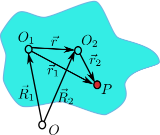
Proving the independence of angular velocity from choice of origin

See the graph to the right: The origin of lab frame is O, while O₁ and O₂ are two fixed points on the rigid body, whose velocity is $\mathbf{v}_1$ and $\mathbf{v}_2$ respectively. Suppose the angular velocity with respect to O₁ and O₂ is $\boldsymbol{\omega}_1$ and $\boldsymbol{\omega}_2$ respectively. Since point P and O₂ have only one velocity,

\mathbf{v}_1 + \boldsymbol{\omega}_1\times\mathbf{r}_1 = \mathbf{v}_2 + \boldsymbol{\omega}_2\times\mathbf{r}_2

\mathbf{v}_2 = \mathbf{v}_1 + \boldsymbol{\omega}_1\times\mathbf{r} = \mathbf{v}_1 + \boldsymbol{\omega}_1\times (\mathbf{r}_1 - \mathbf{r}_2)

The above two yields that

(\boldsymbol{\omega}_1-\boldsymbol{\omega}_2) \times \mathbf{r}_2=0

Since the point P (and thus $\mathbf{r}_2$ ) is arbitrary, it follows that

\boldsymbol{\omega}_1 = \boldsymbol{\omega}_2

If the reference point is the instantaneous axis of rotation the expression of velocity of a point in the rigid body will have just the angular velocity term. This is because the velocity of instantaneous axis of rotation is zero. An example of instantaneous axis of rotation is the hinge of a door. Another example is the point of contact of a purely rolling spherical (or, more generally, convex) rigid body.

References

↑ Hibbeler, Russell C. (2009). Engineering Mechanics. Upper Saddle River, New Jersey: Pearson Prentice Hall. pp. 314, 153. ISBN 978-0-13-607791-6. (EM1)
↑ K.S.HEDRIH: Leonhard Euler (1707–1783) and rigid body dynamics
↑ "online tool to calculate angular speed vectors". Aeroengineering.info. Retrieved 2013-01-23.
↑ Rotations and Angular Momentum on the Classical Mechanics page of the website of John Baez, especially Questions 1 and 2.

Symon, Keith (1971). Mechanics. Addison-Wesley, Reading, MA. ISBN 978-0-201-07392-8.
Landau, L.D.; Lifshitz, E.M. (1997). Mechanics. Butterworth-Heinemann. ISBN 978-0-7506-2896-9.

External links

A college text-book of physics By Arthur Lalanne Kimball (Angular Velocity of a particle)
Pickering, Steve (2009). "ω Speed of Rotation [Angular Velocity]". Sixty Symbols. Brady Haran for the University of Nottingham.

This article is issued from Wikipedia. The text is licensed under Creative Commons - Attribution - Sharealike. Additional terms may apply for the media files.

[EM1-1] Hibbeler, Russell C. (2009). Engineering Mechanics. Upper Saddle River, New Jersey: Pearson Prentice Hall. pp. 314, 153. ISBN 978-0-13-607791-6. (EM1)

[2] K.S.HEDRIH: Leonhard Euler (1707–1783) and rigid body dynamics

[3] "online tool to calculate angular speed vectors". Aeroengineering.info. Retrieved 2013-01-23.

[baez-4] Rotations and Angular Momentum on the Classical Mechanics page of the website of John Baez, especially Questions 1 and 2.