xy is a special package for drawing diagrams. To use it, simply add the following line to the preamble of your document:

\usepackage[all]{xy}

where "all" means you want to load a large standard set of functions from Xy-pic, suitable for developing the kind of diagrams discussed here.

The primary way to draw Xy-pic diagrams is over a matrix-oriented canvas, where each diagram element is placed in a matrix slot:

\xymatrix{A & B \\
          C & D }

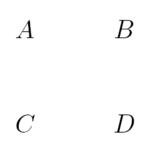
The \xymatrix command puts its contents in math mode. Here, we specified two lines and two columns. To make this matrix a diagram we just add directed arrows using the \ar command.

\xymatrix{ A \ar[r] & B \ar[d] \\
           D \ar[u] & C \ar[l] }

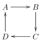
The arrow command is placed on the origin cell for the arrow. The arguments are the direction the arrow should point to (up, down, right and left).

\xymatrix{
    A \ar[d] \ar[dr] \ar[r] & B \\
    D                       & C }

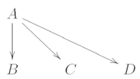
To make diagonals, just use more than one direction. In fact, you can repeat directions to make bigger arrows.

\xymatrix{
    A \ar[d] \ar[dr] \ar[drr] &   &   \\
    B                         & C & D }

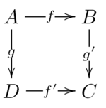
We can draw even more interesting diagrams by adding labels to the arrows. To do this, we use the common superscript and subscript operators.

\xymatrix{
    A \ar[r]^f \ar[d]_g & B \ar[d]^{g'} \\
    D \ar[r]_{f'}       & C }

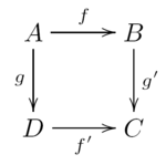
As shown, you use these operators as in math mode. The only difference is that that superscript means "on top of the arrow", and subscript means "under the arrow". There is a third operator, the vertical bar: | It causes text to be placed in the arrow.

\xymatrix{
    A \ar[r]|f \ar[d]|g & B \ar[d]|{g'} \\
    D \ar[r]|{f'}       & C }

To draw an arrow with a hole in it, use \ar[...]|\hole. In some situations, it is important to distinguish between different types of arrows. This can be done by putting labels on them, or changing their appearance

\xymatrix{
    \bullet\ar@{->}[rr]     && \bullet\\
    \bullet\ar@{.<}[rr]     && \bullet\\
    \bullet\ar@{~)}[rr]     && \bullet\\
    \bullet\ar@{=(}[rr]     && \bullet\\
    \bullet\ar@{~/}[rr]     && \bullet\\
    \bullet\ar@{^{(}->}[rr] && \bullet\\
    \bullet\ar@2{->}[rr]    && \bullet\\
    \bullet\ar@3{->}[rr]    && \bullet\\
    \bullet\ar@{=+}[rr]     && \bullet }

Notice the difference between the following two diagrams:

\xymatrix{ \bullet \ar[r] \ar@{.>}[r] & \bullet }

\xymatrix{
    \bullet \ar@/^/[r]
    \ar@/_/@{.>}[r] &
    \bullet }

The modifiers between the slashes define how the curves are drawn. Xy-pic offers many ways to influence the drawing of curves; for more information, check the Xy-pic documentation.

If you are interested in a more thorough introduction then consult the Xy-pic Home Page, which contains links to several other tutorials as well as the reference documentation.