Plotting
There are a number of different packages for plotting in Julia, and there's probably one to suit your needs and tastes. This section is a quick introduction to one of them, Plots.jl, which is interesting because it talks to many of the other plotting packages. Before making plots with Julia, download and install some plotting packages :
(v1.0) pkg> add Plots PyPlot GR UnicodePlots
The first package, Plots, is a high-level plotting package that interfaces with other plotting packages, which here are referred to as 'back-ends'. They act as the graphics "engines" that produce the graphics. Each of these is also a stand-alone plotting package, and can be used separately, but the advantage of using Plots as the interface is, as you'll see, a simpler and consistent interface.
You can start using the Plots.jl package in a Julia session in the usual way:
julia> using Plots
You usually want to plot one or more series, arrays of numerical values. Alternatively, you can provide one or more functions to generate numerical values.
If you want to follow along, the sample data used here is a simple array of numerical values representing the value of the Equation of Time for every day in the current year. (These values were once used to adjust mechanical clocks to account for the erratic orbit of the earth as it wobbles its way around its elliptical orbit.)
julia> using Astro # you'll need to add this package with:  add https://github.com/cormullion/Astro.jl
julia> using Dates
julia> days = Dates.datetime2julian.(Dates.DateTime(2018, 1, 1, 0, 0, 0):Dates.Day(1):Dates.DateTime(2018, 12, 31, 0, 0, 0))
julia> eq_values = map(equation_time, days)
We now have an array of Float64 values, one for each day of the year:
365-element Array{Float64,1}:
 -3.12598
 -3.59633
 -4.97289
 -5.41857
 -5.85688
  ⋮
 -1.08709
 -1.57435
 -2.05845
 -2.53887
 -3.01508
To plot this series, just pass it to Plots' plot() function.
julia> plot(eq_values)
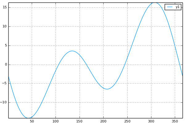
This has used the first available plotting engine. Plots has treated the series as y-values, added other plotting "furniture", automatically provided the x-values to match the y-values you supplied, and then plotted everything for you.
If you want to switch to a different engine, use one of the provided functions: gr(), unicodeplots(), plotly(), and so on. For example, to switch to using the Unicodeplots plotting package (which uses Unicode characters to make plots, and is ideal for use in the REPL/terminal), do this:
julia> unicodeplots()

julia> plot(eq_values)
       +------------------------------------------------------------+
    17 |                                                ,--u        | y1
       |                                              ./   "\       |
       |                                             ./      \      |
       |                                            ./        .     |
       |                                            /         \.    |
       |                                           /           \    |
       |                                          .`           ",   |
       |                                         ,`             \   |
       |                   .r--\.                /               .  |
       |                  /`    \.              /                \  |
       |----------------nr-------fhr-----------v------------------v*|
       |               .F          \.         ,`                  |.|
       |,              /            \,       ,/                    `|
       |l             /              "\.    ,`                      |
       |".           /                 \-ur/`                       |
       | \.         /`                                              |
       |  l        ,`                                               |
       |   \      ./                                                |
       |   "\.  ./`                                                 |
   -15 |     '--"                                                   |
       +------------------------------------------------------------+
       0                                                          370
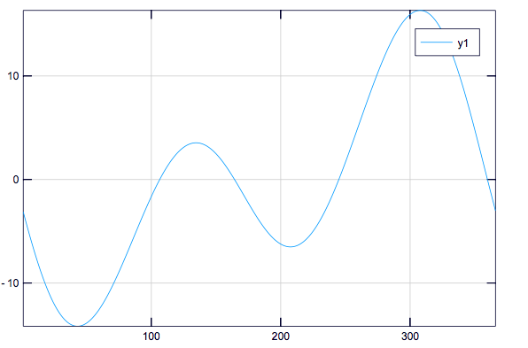
The GR engine/back-end is also a good general purpose plotting package:
julia> gr();
julia> plot(eq_values)
Plotting a function
Switch back to using PyPlot back-end:
julia> pyplot()
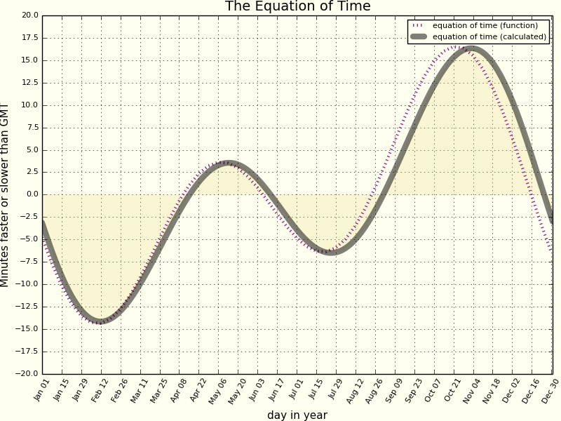
The Equation of Time graph can be approximately modeled by a function combining a couple of sine functions:
julia> equation(d) = -7.65 * sind(d) + 9.87 * sind(2d + 206);
It's easy to plot this function for every day of a year. Pass the function to plot(), and use a range to specify the start and end values:
julia> plot(equation, 1:365)

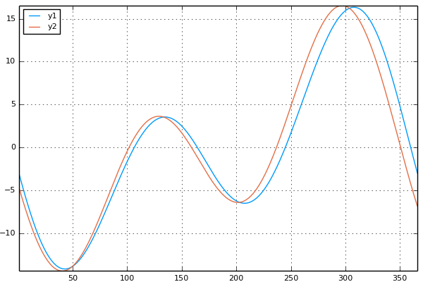
To combine the two plots, so as to compare the equation and the calculated series versions, Plots lets you add another plot to an existing one. The usual Julia convention of using "!" to modify the argument is available here (in an implicit way — you don't actually have to provide the current plot as an argument): the second plot function, plot!() modifies the previous plot:
julia> plot(eq_values);

julia> plot!(equation, 1:365)
Customizing the plots
There is copious documentation for the Plots.jl package, and after studying it you'll be able to spend hours tweaking and customizing your plots to your heart's content. Here are a few examples.
The ticks along the x-axis show the numbers from 1:365, derived automatically from the single series provided. It would be better to see the dates themselves. First, create the strings:
julia> days = Dates.DateTime(2018, 1, 1, 0, 0, 0):Dates.Day(1):Dates.DateTime(2018, 12, 31, 0, 0, 0)
julia> datestrings = Dates.format.(days, "u dd")
The supplied value for the xticks option is a tuple consisting of two arrays/ranges:
(xticks = (1:14:366, datestrings[1:14:366])
the first provides the numerical values, the second provides matching text labels for the ticks.
Extra labels and legends are easily added, and you can access colors from the Colors.jl package. Here's a prettier version of the basic plot:
julia>  plot!(
    eq_values,

    label  = "equation of time (calculated)",
    line=(:black, 0.5, 6, :solid),

    size=(800, 600),

    xticks = (1:14:366, datestrings[1:14:366]),
    yticks = -20:2.5:20,

    ylabel = "Minutes faster or slower than GMT",
    xlabel = "day in year",

    title  = "The Equation of Time",
    xrotation = rad2deg(pi/3),

    fillrange = 0,
    fillalpha = 0.25,
    fillcolor = :lightgoldenrod,

    background_color = :ivory
    )
Other packages
UnicodePlots
If you work in the REPL a lot, perhaps you want a quick and easy way to draw plots that use text rather than graphics for output? The UnicodePlots.jl package uses Unicode characters to draw various plots, avoiding the need to load various graphic libraries. It can produce:
- scatter plots
- line plots
- bar plots (horizontal)
- staircase plots
- histograms (horizontal)
- sparsity patterns
- density plots
Download and add it to your Julia installation, if you haven't already done so:
pkg> add UnicodePlots
You have to do this just once. Now you load the module and import the functions:
julia> using UnicodePlots
Here is a quick example of a line plot:
julia> myPlot = lineplot([1, 2, 3, 7], [1, 2, -5, 7], title="My Plot", border=:dotted)
                       My Plot
      ⡤⠤⠤⠤⠤⠤⠤⠤⠤⠤⠤⠤⠤⠤⠤⠤⠤⠤⠤⠤⠤⠤⠤⠤⠤⠤⠤⠤⠤⠤⠤⠤⠤⠤⠤⠤⠤⠤⠤⠤⠤⢤
   10 ⡇⠀⠀⠀⠀⠀⠀⠀⠀⠀⠀⠀⠀⠀⠀⠀⠀⠀⠀⠀⠀⠀⠀⠀⠀⠀⠀⠀⠀⠀⠀⠀⠀⠀⠀⠀⠀⠀⠀⠀⠀⢸
      ⡇⠀⠀⠀⠀⠀⠀⠀⠀⠀⠀⠀⠀⠀⠀⠀⠀⠀⠀⠀⠀⠀⠀⠀⠀⠀⠀⠀⡠⠄⠀⠀⠀⠀⠀⠀⠀⠀⠀⠀⠀⢸
      ⡇⠀⠀⠀⠀⠀⠀⠀⠀⠀⠀⠀⠀⠀⠀⠀⠀⠀⠀⠀⠀⠀⠀⠀⠀⢀⠔⠊⠀⠀⠀⠀⠀⠀⠀⠀⠀⠀⠀⠀⠀⢸
      ⡇⠀⠀⠀⠀⠀⠀⠀⠀⠀⠀⠀⠀⠀⠀⠀⠀⠀⠀⠀⠀⠀⢀⡠⠊⠁⠀⠀⠀⠀⠀⠀⠀⠀⠀⠀⠀⠀⠀⠀⠀⢸
      ⡇⠀⠀⠀⠀⠔⠒⠊⠉⢣⠀⠀⠀⠀⠀⠀⠀⠀⠀⠀⡠⠔⠁⠀⠀⠀⠀⠀⠀⠀⠀⠀⠀⠀⠀⠀⠀⠀⠀⠀⠀⢸
      ⡇⠉⠉⠉⠉⠉⠉⠉⠉⠉⠫⡉⠉⠉⠉⠉⠉⢉⠝⠋⠉⠉⠉⠉⠉⠉⠉⠉⠉⠉⠉⠉⠉⠉⠉⠉⠉⠉⠉⠉⠁⢸
      ⡇⠀⠀⠀⠀⠀⠀⠀⠀⠀⠀⠱⡀⠀⢀⡠⠊⠁⠀⠀⠀⠀⠀⠀⠀⠀⠀⠀⠀⠀⠀⠀⠀⠀⠀⠀⠀⠀⠀⠀⠀⢸
      ⡇⠀⠀⠀⠀⠀⠀⠀⠀⠀⠀⠀⠑⠔⠁⠀⠀⠀⠀⠀⠀⠀⠀⠀⠀⠀⠀⠀⠀⠀⠀⠀⠀⠀⠀⠀⠀⠀⠀⠀⠀⢸
      ⡇⠀⠀⠀⠀⠀⠀⠀⠀⠀⠀⠀⠀⠀⠀⠀⠀⠀⠀⠀⠀⠀⠀⠀⠀⠀⠀⠀⠀⠀⠀⠀⠀⠀⠀⠀⠀⠀⠀⠀⠀⢸
  -10 ⡇⠀⠀⠀⠀⠀⠀⠀⠀⠀⠀⠀⠀⠀⠀⠀⠀⠀⠀⠀⠀⠀⠀⠀⠀⠀⠀⠀⠀⠀⠀⠀⠀⠀⠀⠀⠀⠀⠀⠀⠀⢸
      ⠓⠒⠒⠒⠒⠒⠒⠒⠒⠒⠒⠒⠒⠒⠒⠒⠒⠒⠒⠒⠒⠒⠒⠒⠒⠒⠒⠒⠒⠒⠒⠒⠒⠒⠒⠒⠒⠒⠒⠒⠒⠚
      0                                       10
And here's a density plot:
julia> myPlot = densityplot(collect(1:100), randn(100), border=:dotted)
      ⡤⠤⠤⠤⠤⠤⠤⠤⠤⠤⠤⠤⠤⠤⠤⠤⠤⠤⠤⠤⠤⠤⠤⠤⠤⠤⠤⠤⠤⠤⠤⠤⠤⠤⠤⠤⠤⠤⠤⠤⠤⢤
   10 ⡇                                        ⢸
      ⡇                                        ⢸
      ⡇                                        ⢸
      ⡇                                        ⢸
      ⡇                                        ⢸
      ⡇                                        ⢸
      ⡇                                        ⢸
      ⡇                            ░           ⢸
      ⡇ ░░░        ░ ▒░  ▒░     ░  ░ ░ ░ ░   ░ ⢸
      ⡇░░  ░▒░░▓▒▒ ▒░░ ▓░░ ░░░▒░ ░ ░   ▒ ░ ░▒░░⢸
      ⡇▓▒█▓▓▒█▓▒▒▒█▒▓▒▓▒▓▒▓▓▒▓▒▓▓▓█▒▒█▓▒▓▓▓▓▒▒▒⢸
      ⡇    ░     ░         ░░░ ░    ▒ ░ ░ ░░ ░ ⢸
      ⡇                          ░             ⢸
      ⡇                                        ⢸
      ⡇                                        ⢸
      ⡇                                        ⢸
      ⡇                                        ⢸
      ⡇                                        ⢸
      ⡇                                        ⢸
  -10 ⡇                                        ⢸
      ⠓⠒⠒⠒⠒⠒⠒⠒⠒⠒⠒⠒⠒⠒⠒⠒⠒⠒⠒⠒⠒⠒⠒⠒⠒⠒⠒⠒⠒⠒⠒⠒⠒⠒⠒⠒⠒⠒⠒⠒⠒⠚
      0                                      100
(Note that it needs the terminal environment for the displayed graphs to be 100% successful - when you copy and paste, some of the magic is lost.)
VegaLite
allows you to create visualizations in a web browser window. VegaLite is a visualization grammar, a declarative format for creating and saving visualization designs. With VegaLite you can describe data visualizations in a JSON format, and generate interactive views using either HTML5 Canvas or SVG. You can produce:
- Area plots
- Bar plots/Histograms
- Line plots
- Scatter plots
- Pie/Donut charts
- Waterfall charts
- Wordclouds
To use VegaLite, first add the package to your Julia installation. You have to do this just once:
pkg> add VegaLite
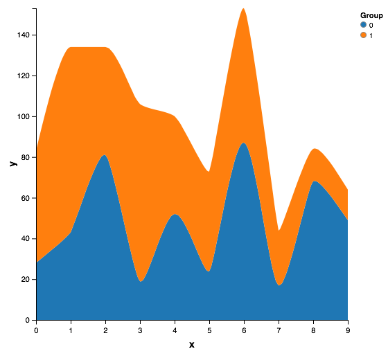
Here's how to create a stacked area plot.
julia> using VegaLite
julia> x = [0,1,2,3,4,5,6,7,8,9,0,1,2,3,4,5,6,7,8,9]
julia> y = [28, 43, 81, 19, 52, 24, 87, 17, 68, 49, 55, 91, 53, 87, 48, 49, 66, 27, 16, 15]
julia> g = [0,0,0,0,0,0,0,0,0,0,1,1,1,1,1,1,1,1,1,1]

julia> a = areaplot(x = x, y = y, group = g, stacked = true)
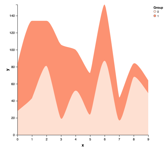
A general feature of VegaLite is that you can modify a visualization after you've created it. So, let's change the color scheme using a function (notice the "!" to indicate that the arguments are modified):
julia> colorscheme!(a, ("Reds", 3))
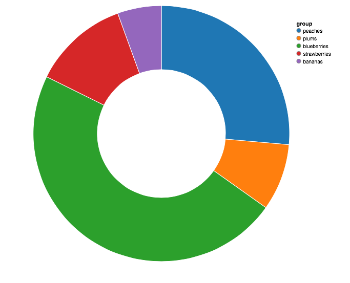
You can create pie (and donut) charts easily by supplying two arrays. The x array provides the labels, the y array provides the quantities:
julia> fruit = ["peaches", "plums", "blueberries", "strawberries", "bananas"];
julia> bushels = [100, 32, 180, 46, 21];
julia> piechart(x = fruit, y = bushels, holesize = 125)