A CORDIC (standing for COordinate Rotation DIgital Computer) circuit serves to compute several common mathematical functions, such as trigonometric, hyperbolic and exponential functions.
Application
A CORDIC uses only adders to compute the result, with the benefit that it can therefore be implemented using relatively basic hardware.
Methods such as power series or table lookups usually need multiplications to be performed. If a hardware multiplier is not available, a CORDIC is generally faster, but if a multiplier can be used, other methods may be faster.
CORDICs can also be implemented in many ways, including a single-stage iterative method, which requires very few gates when compared to multiplier circuits. Also, CORDICs can compute many functions with precisely the same hardware, so they are ideal for applications with an emphasis on reduction of cost (e.g. by reducing gate counts in FPGAs) over speed. An example of this priority is in pocket calculators, where CORDICs are very frequently used.
History
The CORDIC was invented in 1959 by J.E. Volder, in the aeroelectronics departments of Convair, and was designed for the B-58 Hustler bomber's navigational computer to replace an analogue resolver, a device that computed trigonometric functions.
In 1971, J.S. Walther, at Hewlett-Packard, extended the method to calculate hyperbolic and exponential functions, logarithms, multiplications, divisions, and square roots.
General Concept
Consider the following rotations of vectors:
 |
 |
|
|
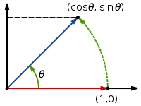
If we were to have a computationally efficient method of rotating a vector, we can directly evaluate sine, cosine and arctan functions. However, rotation by an arbitrary angle is non-trivial (you have to know the sine and cosines, which is precisely what we don't have). We use two methods to make it easier:
- Instead of performing rotations, we perform "pseudorotations", which are easier to compute.
- Construct the desired angle θ from a sum of special angles, αi:

The diagram belows shows a rotation and pseudo-rotation of a vector of length Ri about an angle of ai about the origin:
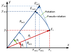
A rotation about the origin produces the following co-ordinates:


Recall the identity .


Our strategy will be to eliminate the factor of and somehow remove the multiplication by . A pseudo-rotation produces a vector with the same angle as the rotated vector, but with a different length. In fact, the pseudo-rotation changes the length to:


Thus we now have these co-ordinates following a pseudo-rotation:


The pseudo-rotation has succeeded in removing our length-factor, which would have required a costly division operation. However, the vector will grow by a factor of K over a sequence of n pseudo-rotations:

The co-ordinates following the n pseudo-rotations are then:


If the angles are always the same set, then K is fixed, and can be accounted for later. We choose these angle according to two criteria:
- We must also choose the angles so that any angle can be constructed from the sum of all them, with appropriate signs.
- We make all a power of 2, so that the multiplication can be performed by a simple logical shift of a binary number.
The tangent function has a monotonically increasing gradient on the interval [0, π/2], so the tangent of a given angle is always less than twice the tangent of half the angle. This means that if we make the angles , we can satify both criteria. Note that the tangent function is odd, which means that to pseudo-rotate the other way, you just subtract, rather than add, the tangent of the angle.

| i | αi = tan−1 (2−i) | |
|---|---|---|
| Degrees | Radians | |
| 0 | 45.00 | 0.7854 |
| 1 | 26.57 | 0.4636 |
| 2 | 14.04 | 0.2450 |
| 3 | 7.13 | 0.1244 |
| 4 | 3.58 | 0.0624 |
| 5 | 1.79 | 0.0312 |
| 6 | 0.90 | 0.0160 |
| 7 | 0.45 | 0.0080 |
| 8 | 0.22 | 0.0040 |
| 9 | 0.11 | 0.0020 |
In step i of the process, we pseudo-rotate by , where is the direction (or sign) of the rotation, which will be chosen at each step to force the angle to converge to the desired final rotation. For example, consider a rotation of 28°:


The more steps we take, the better the approximation that we can make by successive rotations. Thus, we have the following iterative co-ordinate calculation:


In order to achieve k bit of precision, k iterations are needed, because , converging as i increases.

Using CORDICs

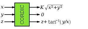
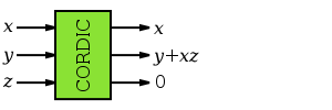
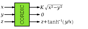
CORDICs can be used to compute many functions. A CORDIC has three inputs, x0, y0, and z0. Depending on the inputs to the CORDIC, various results can be produced at the outputs xn, yn, and zn.
Using CORDIC in rotation mode
|
|
|


For convergence of zn to 0, choose .

If we start with x0 = 1/K and y0=0, at the end of the process, we find xn=cos z0 and yn=sin z0.
The domain of convergence is because 99.7° is the sum of all angles in the list.

Using CORDIC in vectoring mode
|
|
|


For convergence of yn to 0, choose .

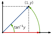
If we start with x0 = 1 and z0 = 0, we find zn=tan−1y0
Implementations of CORDICs
Bit-parallel, unrolled
.svg.png)
Bit-parallel, iterative
.svg.png)
If a high speed is not required, this can be implemented with a single adder and a single shifter.
Bit-serial
The Universal CORDIC
By introducing a factor μ, we can also cater for linear and hyperbolic functions:

Summary of Universal CORDIC implementations
| Mode | Rotation | Vectoring |
|---|---|---|
| Circular
μ = 1 |
 |
 |
| Linear
μ = 0 |
 |
 |
| Hyperbolic
μ = -1 |
 |
 |
| ||


Directly computable functions


Indirectly computable functions
In addition to the above functions, a number of other functions can be produced by combining the results of previous computations:


Further reading
- Volder, J.E. (1959), " The CORDIC trigonometric computing technique", IRE Transactions on Electronic Computers 8 (3): 330–334, http://lapwww.epfl.ch/courses/comparith/Papers/3-Volder_CORDIC.pdf, retrieved 2009-06-02
- Walther, J.S. (1971), "A unified algorithm for elementary functions" (w), Proceedings of the May 18–20, 1971, spring joint computer conference: 379–385, http://portal.acm.org/citation.cfm?id=1478786.1478840, retrieved 2009-06-02
- Vladimir Baykov, Problems of Elementary Functions Evaluation Based on Digit by Digit (CORDIC) Technique, PhD thesis, Leningrad State Univ. of Electrical Eng., 1972
- Schmid, Hermann, Decimal computation. New York, Wiley, 1974
- V.D.Baykov,V.B.Smolov, Hardware implementation of elementary functions in computers, Leningrad State University, 1975, 96p.*Full Text
- Senzig, Don, Calculator Algorithms, IEEE Compcon Reader Digest, IEEE Catalog No. 75 CH 0920-9C, pp139–141, IEEE, 1975.
- V.D.Baykov,S.A.Seljutin, Elementary functions evaluation in microcalculators, Moscow, Radio & svjaz,1982,64p.
- Vladimir D.Baykov, Vladimir B.Smolov, Special-purpose processors: iterative algorithms and structures, Moscow, Radio & svjaz, 1985, 288 pages
- M. E. Frerking, Digital Signal Processing in Communication Systems, 1994
- Vitit Kantabutra, On hardware for computing exponential and trigonometric functions, IEEE Trans. Computers 45 (3), 328-339 (1996)
- Andraka, Ray, A survey of CORDIC algorithms for FPGA based computers
- Henry Briggs, Arithmetica Logarithmica. London, 1624, folio
- CORDIC Bibliography Site, Shaoyun Wang, July 2011
- The secret of the algorithms, Jacques Laporte, Paris 1981
- Digit by digit methods, Jacques Laporte, Paris 2006
- Ayan Banerjee, FPGA realization of a CORDIC based FFT processor for biomedical signal processing, Kharagpur, 2001
- CORDIC Architectures: A Survey, B. Lakshmi and A. S. Dhar, Journal: VLSI Design, January 2010
- Implementation of a CORDIC Algorithm in a Digital Down-Converter, C. Cockrum, Fall 2008
- Parhami, B. (1999), Computer arithmetic: algorithms and hardware designs