In your previous study of calculus, we have looked at functions and their behavior. Most of these functions we have examined have been all in the form

and only occasional examination of functions of two variables. However, the study of functions of several variables is quite rich in itself, and has applications in several fields.
We write functions of vectors - many variables - as follows:

and for the function that maps a vector in to a vector in .


Before we can do calculus in , we must familiarize ourselves with the structure of . We need to know which properties of can be extended to . This page assumes at least some familiarity with basic linear algebra.

Topology in
We are already familiar with the nature of the regular real number line, which is the set , and the two-dimensional plane, . This examination of topology in attempts to look at a generalization of the nature of -dimensional spaces - , or , or .


Lengths and distances
If we have a vector in we can calculate its length using the Pythagorean theorem. For instance, the length of the vector is


We can generalize this to . We define a vector's length, written , as the square root of the sum of the squares of each of its components. That is, if we have a vector ,


Now that we have established some concept of length, we can establish the distance between two vectors. We define this distance to be the length of the two vectors' difference. We write this distance , and it is


This distance function is sometimes referred to as a metric. Other metrics arise in different circumstances. The metric we have just defined is known as the Euclidean metric.
Open and closed balls
In , we have the concept of an interval, in that we choose a certain number of other points about some central point. For example, the interval is centered about the point 0, and includes points to the left and right of 0.
![[-1,1]](../../I/m/51e3b7f14a6f70e614728c583409a0b9a8b9de01.svg)
In and up, the idea is a little more difficult to carry on. For , we need to consider points to the left, right, above, and below a certain point. This may be fine, but for we need to include points in more directions.

We generalize the idea of the interval by considering all the points that are a given, fixed distance from a certain point - now we know how to calculate distances in , we can make our generalization as follows, by introducing the concept of an open ball and a closed ball respectively, which are analogous to the open and closed interval respectively.
- an open ball
- is a set in the form
- a closed ball
- is a set in the form


In , we have seen that the open ball is simply an open interval centered about the point . In this is a circle with no boundary, and in it is a sphere with no outer surface. (What would the closed ball be?)

Boundary points
If we have some area, say a field, then the common sense notion of the boundary is the points 'next to' both the inside and outside of the field. For a set, , we can define this rigorously by saying the boundary of the set contains all those points such that we can find points both inside and outside the set. We call the set of such points .


Typically, when it exists the dimension of is one lower than the dimension of . e.g. the boundary of a volume is a surface and the boundary of a surface is a curve.
This isn't always true; but it is true of all the sets we will be using.
A set is bounded if there is some positive number such that we can encompass this set by a closed ball about . --> if every point in it is within a finite distance of the origin, i.e there exists some such that is in S implies .


Curves and parameterizations
If we have a function , we say that 's image (the set - or some subset of ) is a curve in and is its parametrization.


Parameterizations are not necessarily unique - for example, such that is one parametrization of the unit circle, and such that is a whole family of parameterizations of that circle.


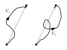
Collision and intersection points
Say we have two different curves. It may be important to consider
- points the two curves share - where they intersect
- intersections which occur for the same value of - where they collide.

Intersection points
Firstly, we have two parameterizations and , and we want to find out when they intersect, this means that we want to know when the function values of each parametrization are the same. This means that we need to solve


because we're seeking the function values independent of the times they intersect.
For example, if we have and , and we want to find intersection points:


with solutions

So, the two curves intersect at the points .

Collision points
However, if we want to know when the points "collide", with and , we need to know when both the function values and the times are the same, so we need to solve instead

For example, using the same functions as before, and , and we want to find collision points:


which gives solutions So the collision points are .

We may want to do this to actually model physical problems, such as in ballistics.
Continuity & differentiability
If we have a parametrization , which is built up out of component functions in the form , is continuous if and only if each component function is also.

In this case the derivative of is
- . This is actually a specific consequence of a more general fact we will see later.

Tangent vectors
Recall in single-variable calculus that on a curve, at a certain point, we can draw a line that is tangent to that curve at exactly at that point. This line is called a tangent. In the several variable case, we can do something similar.
We can expect the tangent vector to depend on and we know that a line is its own tangent, so looking at a parametrised line will show us precisely how to define the tangent vector for a curve.

An arbitrary line is , with: , so


- and
- , which is the direction of the line, its tangent vector.


Similarly, for any curve, the tangent vector is .

Angle between curves
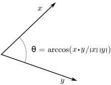
We can then formulate the concept of the angle between two curves by considering the angle between the two tangent vectors. If two curves, parametrized by and intersect at some point, which means that


the angle between these two curves at is the angle between the tangent vectors and is given by


Tangent lines
With the concept of the tangent vector as being analogous to being the gradient of the line in the one variable case, we can form the idea of the tangent line. Recall that we need a point on the line and its direction.
If we want to form the tangent line to a point on the curve, say , we have the direction of the line , so we can form the tangent line


Different parameterizations
One such parametrization of a curve is not necessarily unique. Curves can have several different parametrizations. For example, we already saw that the unit circle can be parametrized by g(t) = (cos at, sin at) such that t ∈ [0, 2π/a).
Generally, if f is one parametrization of a curve, and g is another, with
- f(t0) = g(s0)
there is a function u(t) such that u(t0)=s0, and g'(u(t)) = f(t) near t0.
This means, in a sense, the function u(t) "speeds up" the curve, but keeps the curve's shape.
Surfaces
A surface in space can be described by the image of a function f : R2 → Rn. f is said to be the parametrization of that surface.
For example, consider the function
- f(α, β) = α(2,1,3)+β(-1,2,0)
This describes an infinite plane in R3. If we restrict α and β to some domain, we get a parallelogram-shaped surface in R3.
Surfaces can also be described explicitly, as the graph of a function z = f(x, y) which has a standard parametrization as f(x,y)=(x, y, f(x,y)), or implictly, in the form f(x, y, z)=c.
Level sets
The concept of the level set (or contour) is an important one. If you have a function f(x, y, z), a level set in R3 is a set of the form {(x,y,z)|f(x,y,z)=c}. Each of these level sets is a surface.
Level sets can be similarly defined in any Rn
Level sets in two dimensions may be familiar from maps, or weather charts. Each line represents a level set. For example, on a map, each contour represents all the points where the height is the same. On a weather chart, the contours represent all the points where the air pressure is the same.
Limits and continuity
Before we can look at derivatives of multivariate functions, we need to look at how limits work with functions of several variables first, just like in the single variable case.
If we have a function f : Rm → Rn, we say that f(x) approaches b (in Rn) as x approaches a (in Rm) if, for all positive ε, there is a corresponding positive number δ, |f(x)-b| < ε whenever |x-a| < δ, with x ≠ a.
This means that by making the difference between x and a smaller, we can make the difference between f(x) and b as small as we want.
If the above is true, we say
- f(x) has limit b at a
- f(x) approaches b as x approaches a
- f(x) → b as x → a

These four statements are all equivalent.
Rules
Since this is an almost identical formulation of limits in the single variable case, many of the limit rules in the one variable case are the same as in the multivariate case.
For f and g, mapping Rm to Rn, and h(x) a scalar function mapping Rm to R, with
- f(x) → b as x → a
- g(x) → c as x → a
- h(x) → H as x → a
then:


and consequently


when H≠0

Continuity
Again, we can use a similar definition to the one variable case to formulate a definition of continuity for multiple variables.
If f : Rm → Rn, f is continuous at a point a in Rm if f(a) is defined and

Just as for functions of one dimension, if f, g are both continuous at p, f+g, λf (for a scalar λ), f·g, and f×g are continuous also. If φ : Rm → R is continus at p, φf, f/φ are too if φ is never zero.
From these facts we also have that if A is some matrix which is n×m in size, with x in Rm, a function f(x)=A x is continuous in that the function can be expanded in the form x1a1+...+xmam, which can be easily verified from the points above.
If f : Rm → Rn which is in the form f(x) = (f1(x),...,fn(x) is continuous if and only if each of its component functions are a polynomial or rational function, whenever they are defined.
Finally, if f is continuous at p, g is continuous at f(p), g(f(x)) is continuous at p.
Special note about limits
It is important to note that we can approach a point in more than one direction, and thus, the direction that we approach that point counts in our evaluation of the limit. It may be the case that a limit may exist moving in one direction, but not in another.
Differentiable functions
We will start from the one-variable definition of the derivative at a point p, namely

Let's change above to equivalent form of

which achieved after pulling f'(p) inside and putting it over a common denominator.
We can't divide by vectors, so this definition can't be immediately extended to the multiple variable case. Nonetheless, we don't have to: the thing we took interest in was the quotient of two small distances (magnitudes), not their other properties (like sign). It's worth noting that 'other' property of vector neglected is its direction. Now we can divide by the absolute value of a vector, so lets rewrite this definition in terms of absolute values

Another form of formula above is obtained by letting we have and if , the , so


- ,

where can be thought of as a 'small change'.

So, how can we use this for the several-variable case?
If we switch all the variables over to vectors and replace the constant (which performs a linear map in one dimension) with a matrix (which denotes also a linear map), we have

or

If this limit exists for some f : Rm → Rn, and there is a linear map A : Rm → Rn (denoted by matrix A which is m×n), we refer to this map as being the derivative and we write it as Dp f.
A point on terminology - in referring to the action of taking the derivative (giving the linear map A), we write Dp f, but in referring to the matrix A itself, it is known as the Jacobian matrix and is also written Jp f. More on the Jacobian later.
Properties
There are a number of important properties of this formulation of the derivative.
Affine approximations
If f is differentiable at p for x close to p, |f(x)-(f(p)+A(x-p))| is small compared to |x-p|, which means that f(x) is approximately equal to f(p)+A(x-p).
We call an expression of the form g(x)+c affine, when g(x) is linear and c is a constant. f(p)+A(x-p) is an affine approximation to f(x).
Jacobian matrix and partial derivatives
The Jacobian matrix of a function is in the form

for a f : Rm → Rn, Jp f' is a n×m matrix.
The consequence of this is that if f is differentiable at p, all the partial derivatives of f exist at p.
However, it is possible that all the partial derivatives of a function exist at some point yet that function is not differentiable there, so it is very important not to mix derivative (linear map) with the Jacobian (matrix) especially in situations akin to the one cited.
Continuity and differentiability
Furthermore, if all the partial derivatives exist, and are continuous in some neighbourhood of a point p, then f is differentiable at p. This has the consequence that for a function f which has its component functions built from continuous functions (such as rational functions, differentiable functions or otherwise), f is differentiable everywhere f is defined.
We use the terminology continuously differentiable for a function differentiable at p which has all its partial derivatives existing and are continuous in some neighbourhood at p.
Rules of taking Jacobians
If f : Rm → Rn, and h(x) : Rm → R are differentiable at 'p':


Important: make sure the order is right - matrix multiplication is not commutative!
Chain rule
The chain rule for functions of several variables is as follows. For f : Rm → Rn and g : Rn → Rp, and g o f differentiable at p, then the Jacobian is given by

Again, we have matrix multiplication, so one must preserve this exact order. Compositions in one order may be defined, but not necessarily in the other way.
Alternate notations
For simplicity, we will often use various standard abbreviations, so we can write most of the formulae on one line. This can make it easier to see the important details.
We can abbreviate partial differentials with a subscript, e.g.,

When we are using a subscript this way we will generally use the Heaviside D rather than ∂,

Mostly, to make the formulae even more compact, we will put the subscript on the function itself.

If we are using subscripts to label the axes, x1, x2 …, then, rather than having two layers of subscripts, we will use the number as the subscript.

We can also use subscripts for the components of a vector function, u=(ux, uy, uy) or u=(u1,u2…un)
If we are using subscripts for both the components of a vector and for partial derivatives we will separate them with a comma.

The most widely used notation is hx. Both h1 and ∂1h are also quite widely used whenever the axes are numbered. The notation ∂xh is used least frequently.
We will use whichever notation best suits the equation we are working with.
Directional derivatives
Normally, a partial derivative of a function with respect to one of its variables, say, xj, takes the derivative of that "slice" of that function parallel to the xj'th axis.
More precisely, we can think of cutting a function f(x1,...,xn) in space along the xj'th axis, with keeping everything but the xj variable constant.
From the definition, we have the partial derivative at a point p of the function along this slice as

provided this limit exists.
Instead of the basis vector, which corresponds to taking the derivative along that axis, we can pick a vector in any direction (which we usually take as being a unit vector), and we take the directional derivative of a function as

where d is the direction vector.
If we want to calculate directional derivatives, calculating them from the limit definition is rather painful, but, we have the following: if f : Rn → R is differentiable at a point p, |p|=1,

There is a closely related formulation which we'll look at in the next section.
Gradient vectors
The partial derivatives of a scalar tell us how much it changes if we move along one of the axes. What if we move in a different direction?
We'll call the scalar f, and consider what happens if we move an infintesimal direction dr=(dx,dy,dz), using the chain rule.

This is the dot product of dr with a vector whose components are the partial derivatives of f, called the gradient of f

We can form directional derivatives at a point p, in the direction d then by taking the dot product of the gradient with d
- .

Notice that grad f looks like a vector multiplied by a scalar. This particular combination of partial derivatives is commonplace, so we abbreviate it to

We can write the action of taking the gradient vector by writing this as an operator. Recall that in the one-variable case we can write d/dx for the action of taking the derivative with respect to x. This case is similar, but ∇ acts like a vector.
We can also write the action of taking the gradient vector as:

Properties of the gradient vector
Geometry
- Grad f(p) is a vector pointing in the direction of steepest slope of f. |grad f(p)| is the rate of change of that slope at that point.
For example, if we consider h(x, y)=x2+y2. The level sets of h are concentric circles, centred on the origin, and

grad h points directly away from the origin, at right angles to the contours.
- Along a level set, (∇f)(p) is perpendicular to the level set {x|f(x)=f(p) at x=p}.
If dr points along the contours of f, where the function is constant, then df will be zero. Since df is a dot product, that means that the two vectors, df and grad f, must be at right angles, i.e. the gradient is at right angles to the contours.
Algebraic properties
Like d/dx, ∇ is linear. For any pair of constants, a and b, and any pair of scalar functions, f and g

Since it's a vector, we can try taking its dot and cross product with other vectors, and with itself.
Divergence
If the vector function u maps Rn to itself, then we can take the dot product of u and ∇. This dot product is called the divergence.

If we look at a vector function like v=(1+x2,xy) we can see that to the left of the origin all the v vectors are converging towards the origin, but on the right they are diverging away from it.
Div u tells us how much u is converging or diverging. It is positive when the vector is diverging from some point, and negative when the vector is converging on that point.
- Example:
- For v=(1+x2, xy), div v=3x, which is positive to the right of the origin, where v is diverging, and negative to the left of the origin, where v is converging.
Like grad, div is linear.

Later in this chapter we will see how the divergence of a vector function can be integrated to tell us more about the behaviour of that function.
To find the divergence we took the dot product of ∇ and a vector with ∇ on the left. If we reverse the order we get

To see what this means consider i·∇ This is Dx, the partial differential in the i direction. Similarly, u·∇ is the partial differential in the u direction, multiplied by |u|
Curl
If u is a three-dimensional vector function on R3 then we can take its cross product with ∇. This cross product is called the curl.

Curl u tells us if the vector u is rotating round a point. The direction of curl u is the axis of rotation.
We can treat vectors in two dimensions as a special case of three dimensions, with uz=0 and Dzu=0. We can then extend the definition of curl u to two-dimensional vectors

This two dimensional curl is a scalar. In four, or more, dimensions there is no vector equivalent to the curl.
Example:
Consider u=(-y, x). These vectors are tangent to circles centred on the origin, so appear to be rotating around it anticlockwise.

Example
Consider u=(-y, x-z, y), which is similar to the previous example.

This u is rotating round the axis i+k
Later in this chapter we will see how the curl of a vector function can be integrated to tell us more about the behaviour of that function.
Product and chain rules
Just as with ordinary differentiation, there are product rules for grad, div and curl.
- If g is a scalar and v is a vector, then
- the divergence of gv is
-
- the curl of gv is


- If u and v are both vectors then
- the gradient of their dot product is
-
- the divergence of their cross product is
-
- the curl of their cross product is


We can also write chain rules. In the general case, when both functions are vectors and the composition is defined, we can use the Jacobian defined earlier.

where Ju is the Jacobian of u at the point v.
Normally J is a matrix but if either the range or the domain of u is R1 then it becomes a vector. In these special cases we can compactly write the chain rule using only vector notation.
- If g is a scalar function of a vector and h is a scalar function of g then

- If g is a scalar function of a vector then

This substitution can be made in any of the equations containing ∇
Second order differentials
We can also consider dot and cross products of ∇ with itself, whenever they can be defined. Once we know how to simplify products of two ∇'s we'll know out to simplify products with three or more.
The divergence of the gradient of a scalar f is

This combination of derivatives is the Laplacian of f. It is commmonplace in physics and multidimensional calculus because of its simplicity and symmetry.
We can also take the Laplacian of a vector,

The Laplacian of a vector is not the same as the divergence of its gradient

Both the curl of the gradient and the divergence of the curl are always zero.

This pair of rules will prove useful.
Integration
We have already considered differentiation of functions of more than one variable, which leads us to consider how we can meaningfully look at integration.
In the single variable case, we interpret the definite integral of a function to mean the area under the function. There is a similar interpretation in the multiple variable case: for example, if we have a paraboloid in R3, we may want to look at the integral of that paraboloid over some region of the xy plane, which will be the volume under that curve and inside that region.
Riemann sums
When looking at these forms of integrals, we look at the Riemann sum. Recall in the one-variable case we divide the interval we are integrating over into rectangles and summing the areas of these rectangles as their widths get smaller and smaller. For the multiple-variable case, we need to do something similar, but the problem arises how to split up R2, or R3, for instance.
To do this, we extend the concept of the interval, and consider what we call a n-interval. An n-interval is a set of points in some rectangular region with sides of some fixed width in each dimension, that is, a set in the form {x∈Rn|ai ≤ xi ≤ bi with i = 0,...,n}, and its area/size/volume (which we simply call its measure to avoid confusion) is the product of the lengths of all its sides.
So, an n-interval in R2 could be some rectangular partition of the plane, such as {(x,y) | x ∈ [0,1] and y ∈ [0, 2]|}. Its measure is 2.
If we are to consider the Riemann sum now in terms of sub-n-intervals of a region Ω, it is

where m(Si) is the measure of the division of Ω into k sub-n-intervals Si, and x*i is a point in Si. The index is important - we only perform the sum where Si falls completely within Ω - any Si that is not completely contained in Ω we ignore.
As we take the limit as k goes to infinity, that is, we divide up Ω into finer and finer sub-n-intervals, and this sum is the same no matter how we divide up Ω, we get the integral of f over Ω which we write

For two dimensions, we may write

and likewise for n dimensions.
Iterated integrals
Thankfully, we need not always work with Riemann sums every time we want to calculate an integral in more than one variable. There are some results that make life a bit easier for us.
For R2, if we have some region bounded between two functions of the other variable (so two functions in the form f(x) = y, or f(y) = x), between a constant boundary (so, between x = a and x =b or y = a and y = b), we have

An important theorem (called Fubini's theorem) assures us that this integral is the same as
- ,
if f is continuous on the domain of integration.
Order of integration
In some cases the first integral of the entire iterated integral is difficult or impossible to solve, therefore, it can be to our advantage to change the order of integration.


As of the writing of this, there is no set method to change an order of integration from dxdy to dydx or some other variable. Although, it is possible to change the order of integration in an x and y simple integration by simply switching the limits of integration around also, in non-simple x and y integrations the best method as of yet is to recreate the limits of the integration from the graph of the limits of integration.
In higher order integration that can't be graphed, the process can be very tedious. For example, dxdydz can be written into dzdydx, but first dxdydz must be switched to dydxdz and then to dydzdx and then to dzdydx (as 3-dimensional cases can be graphed, this method would lack parsimony).
Parametric integrals
If we have a vector function, u, of a scalar parameter, s, we can integrate with respect to s simply by integrating each component of u separately.

Similarly, if u is given a function of vector of parameters, s, lying in Rn, integration with respect to the parameters reduces to a multiple integral of each component.
Line integrals
In higher dimensions, saying we are integrating from a to b is not sufficient. In general, we must also specify the path taken between a and b.
We can then write the integrand as a function of the arclength along the curve, and integrate by components.
E.g., given a scalar function h(r) we write

where C is the curve being integrated along, and t is the unit vector tangent to the curve.
There are some particularly natural ways to integrate a vector function, u, along a curve,

where the third possibility only applies in 3 dimensions.
Again, these integrals can all be written as integrals with respect to the arclength, s.

If the curve is planar and u a vector lying in the same plane, the second integral can be usefully rewritten. Say,

where t, n, and b are the tangent, normal, and binormal vectors uniquely defined by the curve.
Then

For the 2-d curves specified b is the constant unit vector normal to their plane, and ub is always zero.
Therefore, for such curves,

Green's Theorem
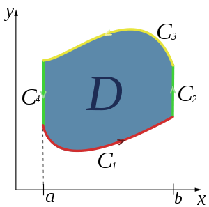
Let C be a piecewise smooth, simple closed curve that bounds a region S on the Cartesian plane. If two function M(x,y) and N(x,y) are continuous and their partial derivatives are continuous, then

In order for Green's theorem to work there must be no singularities in the vector field within the boundaries of the curve.
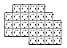
Green's theorem works by summing the circulation in each infinitesimal segment of area enclosed within the curve.

To show how an infinitesimal loop satisfies Green's theorem, consider the infinitesimal rectangle . Let be an arbitrary point inside the rectangle, and let be the counterclockwise boundary of .
![{\displaystyle R=[x_{l},x_{u}]\times [y_{l},y_{u}]}](../../I/m/bf72fdd0b1dd1e8007d785f14f9fc4b5f48419fd.svg)


The circulation around is approximately (the error vanishes as ):


As , the relative errors present in the approximations vanish, and therefore, for an infinitesimal rectangle,

Adding together a family of infinitesimal loops demonstrates Green's theorem for a single large loop.
Inverting differentials
We can use line integrals to calculate functions with a specified gradient:
- If grad V = u
- where h is any function of zero gradient and curl u must be zero.

For example, if V=r2 then

and
![{\begin{matrix}\int _{{{\mathbf {0}}}}^{{{\mathbf {r}}}}2{\mathbf {u}}\cdot d{\mathbf {u}}&=&\int _{{{\mathbf {0}}}}^{{{\mathbf {r}}}}2\left(udu+vdv+wdw\right)\\&=&\left[u^{2}\right]_{{{\mathbf {0}}}}^{{{\mathbf {r}}}}+\left[v^{2}\right]_{{{\mathbf {0}}}}^{{{\mathbf {r}}}}+\left[w^{2}\right]_{{{\mathbf {0}}}}^{{{\mathbf {r}}}}\\&=&x^{2}+y^{2}+z^{2}=r^{2}\\\end{matrix}}](../../I/m/c5f80c2b7342cf136230ed4bca28dc78541abf8d.svg)
so this line integral of the gradient gives the original function.
We will soon see that this integral does not depend on the path, apart from a constant.
Surface and Volume Integrals
Just as with curves, it is possible to parameterise surfaces then integrate over those parameters without regard to geometry of the surface.
That is, to integrate a scalar function V over a surface A parameterised by r and s we calculate

where J is the Jacobian of the transformation to the parameters.
To integrate a vector this way, we integrate each component separately.
However, in three dimensions, every surface has an associated normal vector n, which can be used in integration. We write dS=ndS.
For a scalar function, V, and a vector function, v, this gives us the integrals

These integrals can be reduced to parametric integrals but, written this way, it is clear that they reflect more of the geometry of the surface.
When working in three dimensions, dV is a scalar, so there is only one option for integrals over volumes.
Surface Vectors
Consider an infinitesimal surface element with an area of and a unit outwards normal vector of . The infinitesimal "surface vector" describes the infinitesimal surface element in a manner similar to how the infinitesimal displacement describes an infinitesimal portion of a path. More specifically, similar to how the interior points on a path do not affect the total displacement, the interior points on a surface to not affect the total surface vector.


Consider for instance two paths and that both start at point , and end at point . The total displacements, and , are both equivalent and equal to the displacement between and . Note however that the total lengths and are not necessarily equivalent.


Similarly, given two surfaces and that both share the same counter-clockwise oriented boundary , the total surface vectors and are both equivalent and are a function of the boundary . This implies that a surface can be freely deformed within its boundaries without changing the total surface vector. Note however that the surface areas and are not necessarily equivalent.


The fact that the total surface vectors of and are equivalent is not immediately obvious. To prove this fact, let be a constant vector field. and share the same boundary, so the flux/flow of through and is equivalent. The flux through is , and similarly for is . Since for every choice of , it follows that .


The geometric significance of the total surface vector is that each component measures the area of the projection of the surface onto the plane formed by the other two dimensions. Let be a surface with surface vector . It is then the case that: is the area of the projection of onto the yz-plane; is the area of the projection of onto the xz-plane; and is the area of the projection of onto the xy-plane.


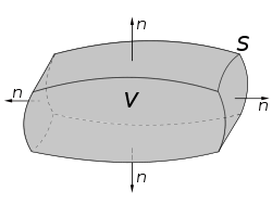
Gauss's divergence theorem
We know that, in one dimension,

Integration is the inverse of differentiation, so integrating the differential of a function returns the original function.
This can be extended to two or more dimensions in a natural way, drawing on the analogies between single variable and multivariable calculus.
The analog of D is ∇, so we should consider cases where the integrand is a divergence.
Instead of integrating over a one-dimensional interval, we need to integrate over a n-dimensional volume.
In one dimension, the integral depends on the values at the edges of the interval, so we expect the result to be connected with values on the boundary.
This suggests a theorem of the form,

This is indeed true, for vector fields in any number of dimensions.
This is called Gauss's theorem.
There are two other, closely related, theorems for grad and curl:
- ,

- ,

with the last theorem only being valid where curl is defined.
These 3 formulas which relate volume integrals to corresponding surface integrals can be proven by decomposing a large volume into a family of infinitesimal volumes, and demonstrating each formula for an infinitesimal volume. In this case the volumes will be assumed to be infinitesimal rectangular prisms. Let be an infinitesimal rectangular prism, where , , and . Let be an arbitrary point inside the rectangular prism, and let denote the outwards oriented surface of .
![{\displaystyle R=[x_{l},x_{u}]\times [y_{l},y_{u}]\times [z_{l},z_{u}]}](../../I/m/65801ccb2863ca3f3a8fd6053d5b17b6fc439f43.svg)


With respect to Gauss's Divergence theorem (the relative error in the approximations vanish as ),


Therefore Gauss's divergence theorem holds for an infinitesimal rectangular prism, and by combining a family of infinitesimal rectangular prisms, holds for an arbitrary volume as well.
For the gradient version,


Therefore for an infinitesimal rectangular prism,

For the curl version,


Therefore for an infinitesimal rectangular prism,

Stokes' curl theorem
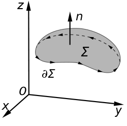
These theorems also hold in two dimensions, where they relate surface and line integrals. Gauss's divergence theorem becomes

where s is arclength along the boundary curve and the vector n is the unit normal to the curve that lies in the surface S, i.e. in the tangent plane of the surface at its boundary, which is not necessarily the same as the unit normal associated with the boundary curve itself.
Similarly, we get
- ,

where C is the boundary of S
In this case the integral does not depend on the surface S.
To see this, suppose we have different surfaces, S1 and S2, spanning the same curve C, then by switching the direction of the normal on one of the surfaces we can write

The left hand side is an integral over a closed surface bounding some volume V so we can use Gauss's divergence theorem.

but we know this integrand is always zero so the right hand side of (2) must always be zero, i.e. the integral is independent of the surface.
This means we can choose the surface so that the normal to the curve lying in the surface is the same as the curves intrinsic normal.
Then, if u itself lies in the surface, we can write

just as we did for line integrals in the plane earlier, and substitute this into (1) to get

This is Stokes' curl theorem